SPL Simplified SQL - Multilayer Fixed Grouping
In the development of database application, we often need to face all kinds of complex SQL computing, one of which is multi-layer fixed grouping. The idea of this algorithm is to align the source data according to the fixed basis with the left join statement, but because the algorithm often involves grouping and aggregation, inter-line calculation, filling missing data, and there are many levels, the corresponding SQL statements will be very complex.
This article will introduce a relatively simple and understandable method, that is, using SPL to achieve multi-layer fixed grouping. Here's an example:
Table stocklog stores records of multiple entries and exits of various goods per day. Some of the data in the table are as follows:
IDate |
Iname |
Iquantity |
Indicator |
2014-04-01 |
Item1 |
15 |
|
2014-04-01 |
Item1 |
4 |
|
2014-04-02 |
Item1 |
3 |
|
2014-04-02 |
Item1 |
10 |
ISSUE |
2014-04-03 |
Item1 |
3 |
|
2014-04-04 |
Item1 |
5 |
ISSUE |
2014-04-07 |
Item1 |
4 |
|
2014-04-10 |
Item1 |
2 |
ISSUE |
2014-04-01 |
Item2 |
20 |
|
2014-04-02 |
Item3 |
30 |
|
2014-04-03 |
Item3 |
14 |
ISSUE |
The expected result is to list the inventory status of each item every day for a specified period of time. Among them, inventory status refers to the number of products open, Enter, Total, Issued and Close each day. As shown in the following figure:
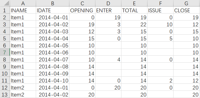
In the original table data, if the value of Indicator is empty, it means that the record is an inbound action, and if it is ISSUE, it means an outbound action. At the same time, it should be noted that the actual record date may be missing, that is, there is no entry and exit record at all for a few days, but for the statistical inventory status, it must include a complete continuous date, and meet the following rules: the "Open" of the day should be equal to the "Close" of the previous day, "Enter" and "Issued" are from the table stocklog, "Total" is equal to "Open+Enter", "Close" is equal to "Open+Enter-Issued" or "Total-Issued".
The SPL codes are as follows:
A |
B |
|
1 |
=db.query("select IDATE, INAME, sum(CASE INDICATOR WHEN'ISSUE'THEN 0 ELSE IQUANTITY END) ENTER, sum(CASE INDICATOR WHEN'ISSUE'THEN IQUANTITY ELSE 0 END) ISSUE from stocklog where IDATE >= ? and IDATE <= ? group by IDATE, INAME",start,end) |
|
2 |
=A1.group(INAME) |
=periods(start,end,1) |
3 |
for A2 |
=A3.align(B2,IDATE) |
4 |
>c=0 |
|
5 |
=B3.new(A3.INAME,B2(#):IDATE, c:OPENING, ENTER,(b=c+ENTER):TOTAL,ISSUE,(c=b-ISSUE):CLOSE) |
|
6 |
=@|B5 |
|
7 |
>file("stocklog.xlsx").xlsexport@t(B6) |
|
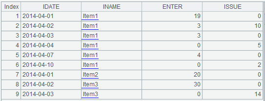
A1: Query the database and calculate the total number of entry and exit of each product every day according to the table stocklog. Here, we only need to group and aggregate the data. There is no difficulty in calculation, and we can leave the task to the SQL statement to complete. It is worth noting that there are two parameters in A1, start and end, which correspond to the two question marks in the SQL statement respectively. They represent the time period passed in from outside, either from JAVA or reporting tool. Assuming that the values of start and end are 2014-04-01 and 2014-04-10 respectively, the results of A1 calculation are as follows:
A2=A1.group(INAME)
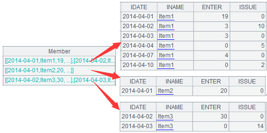
This code divides A1 into groups according to INAME, and each group of data is the entered and issued quantity of each day in the specified time period for a product. It is worth noting that there is no need to aggregate the data after grouping, that is to say, it is a pure grouping operation. The results of A2 calculation are as the left side of the following figure, and on the right side are the details of each group of data.
For grouping, esProc SPL has two functions: groups and group. Function groups is similar to group by statement in SQL, which can be aggregated while grouping. The group function only groups, and does not aggregate, this pure grouping function is lacking in SQL.
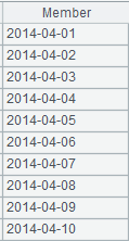
The final calculation result is the inventory status of each day between start and end, and the source data does not record the entries and exits every day, so A2 should be aligned according to the continuous time series. The following is the time series.
B2=periods(start,end,1)
Function periods can generate time series with three parameters: start time, end time and interval. By default, the date series will be generated, and the time series of year, quarter, month and ten days can also be generated with the option. The calculation results of A3 are as follows:
A3=for A2, this is a loop statement, which means that A2 is looped and one product is calculated at a time.
B3-B6 is the loop body. The specific algorithm is to align the product's entry and exit records with the time series in B2, then calculate the daily inventory status of each product, and finally add the calculation results to B6. It is noteworthy that esProc uses intuitive indentation to represent the loop body, rather than brackets or begin/end identifiers. B3-B6 is the loop body of loop statement A3.
B3=A3.align(B2,IDATE)
This code aligns the entry and exit records of the current product with the time series in B2. Note that A3 is both a loop statement and a loop variable, i.e. the entry and exit records of the current product. Take Item3 as an example, the data before alignment is on the left and after alignment is on the right of the following figure:
|
|
B4>c=0
This code is used to assign an initial value of 0 to variable c. c represents the OPENING field of each inventory status of the current product, the OPENING field of the initial date is 0, and c will be constantly modified in B5.
B5=B3.new(A3.INAME:INAME,B2(#):IDATE, c:OPENING, ENTER,(b=c+ENTER):TOTAL,ISSUE,(c=b-ISSUE):CLOSE)
This code is used to calculate inventory status, which is the core of the whole calculation process. B3.new(…) generates a new table based on B3, that is, the inventory status of the current product. There are seven fields in the new table, which are:
A3. INAME: INAME ----Take out the INAME field from the current product's warehouse entry and exit record A3, and the new field is called INAME.
B2 (#):IDATE ----The time series B2 is inserted into the new table in order as the new field IDATE. Note that # denotes the record serial number of A3, and B2 (N) denotes the N record of B2, so B2(#) denotes inserting B2 into the new table according to the serial number of A3.
c: OPENING ----The variable c is used as the field value of OPENING, which is 0 for the first record.
ENTER----The field ENTER in B3 is treated as a new field directly. Because the new table is based on B3, there is no need to rename it like the INAME field.
(b=c+ENTER):TOTAL----The field TOTAL is calculated according to the formula OPENING+ENTER. For clarity, the expression is enclosed in brackets.
ISSUE---Use the field ISSUE in B3 as the new field directly.
(c=b-ISSUE):CLOSE---The CLOSE field is calculated according to the formula TOTAL-ISSUE. Note that the c here has been modified, and when calculating the next record, c will be used as the value of the OPENING field to satisfy the business rule that the "Open" of the day is equal to the "Close" of the previous day.
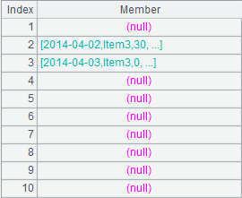
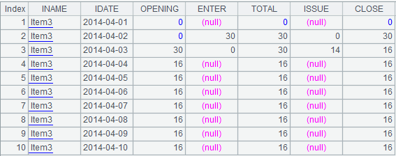
Taking Item3 as an example, the calculation results of B5 are as follows:
B6=@|B5
This code continuously adds B5 to the current grid, @ denotes the current grid B6, and the final result is as follows:
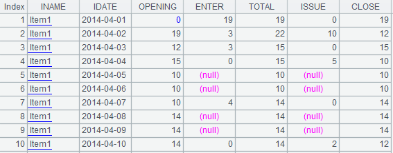
B6 is the final result of this example.
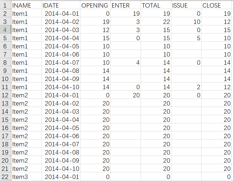
>file("stocklog.xlsx").xlsexport@t(B6)
This code exports the calculation results to the "stocklog. xlsx" file, which can be viewed through the excel tool:
In addition, esProc can be invoked by reporting tool or Java program, and the method of invocation is similar to that of ordinary database. The JDBC interface provided by esProc can return the result of calculation in the form of ResultSet to the Java main program. The specific method can refer to the relevant documents.【How to call an SPL script in Java】
SPL Official Website 👉 http://www.scudata.com
SPL Feedback and Help 👉 https://www.reddit.com/r/esProc
SPL Learning Material 👉 http://c.scudata.com
SPL Source Code and Package 👉 https://github.com/SPLWare/esProc
Discord 👉 https://discord.gg/ydhVnFH9
Youtube 👉 https://www.youtube.com/@esProc_SPL


