Group Excel Data and List Column Values Horizontally in Specific Order
Here’s an Excel file storing stock return data:
| A |
B |
|
| 1 |
Date |
Stock_Return |
| 2 |
1995-01-01 |
-5.20% |
| 3 |
1995-02-01 |
2.10% |
| 4 |
1995-03-01 |
3.70% |
| 5 |
1995-04-01 |
6.90% |
| 6 |
1995-05-01 |
6.50% |
| 7 |
1995-06-01 |
-5.60% |
| 8 |
1995-07-01 |
6.60% |
| 9 |
1995-08-01 |
6.20% |
Task: Group Stock_Return column by segment according to the interval [-∞,-0.07,-0.05,-0.03,0,0.03,0.05,0.07], list the corresponding dates horizontally by Stock_Return values in ascending order, and enter the result to the right of the original Excel data, as shown below:
| D |
E |
F |
G |
H |
|
| 1 |
-Infinity to -0.07 |
||||
| 2 |
-0.07 to -0.05 |
1995-06-01 |
1995-01-01 |
||
| 3 |
-0.05 to -0.03 |
||||
| 4 |
-0.03 to 0 |
||||
| 5 |
0 to 0.03 |
1995-02-01 |
|||
| 6 |
0.03 to 0.05 |
1995-03-01 |
|||
| 7 |
0.05 to 0.07 |
1995-08-01 |
1995-05-01 |
1995-07-01 |
1995-04-01 |
Though it’s a little hard to group the data by segment, Excel is able to manage it. The tough nut to crack is to list dates horizontally in the specific order.
Directions:
1. Start esProc (Download esProc installation package and free DSK edition license HERE. You will be prompted to load the license file when you run esProc for the first time).
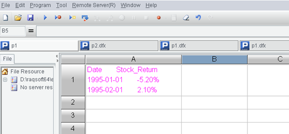
2. Open the to-be-processed file in Excel, select the area of A1:B9, and press Ctrl+C to copy the selected area to clipboard.
3. Open esProc, select cell A1, and press Ctrl+V to paste data from the clipboard to A1. Make sure that the caret is placed above A1 in its editing status during the pasting.

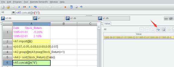
4. Go on with editing the script in esProc:
| A |
|
| 1 |
…( Data pasted from the clipboard ) |
| 2 |
=A1.import@t() |
| 3 |
=[-0.07,-0.05,-0.03,0,0.03,0.05,0.07] |
| 4 |
=A2.group@n(A3.pseg(Stock_Return)+1) |
| 5 |
=A4.(~.sort(Stock_Return).(Date)) |
| 6 |
=A5.concat@n("\t") |
The script function group()divides rows into groups but won’t summarize them; @n option enables a grouping operation by segment number beginning from 1. pseg() function returns the segment number corresponding to the current value; the value begins from 1 by default. concat() function concatenate members of each sub-sequence in a sequence into a string; @n option enables using carriage return to separate strings.
5. Press F9 to execute the esProc script. Then you can click A6 to view the result in the value viewing section on the right. Click the “Copy data” button on the right-hand to paste A6’s result to clipboard.

6. Select cell E1 in Excel and press Ctrl+V to populate the result to the area of E1:H7.
7. We also have column D in the Excel file, which is the leftmost headers, waiting to be handled. You can enter values manually, or write the following script in esProc and then use same method to copy and paste A8’s result to column D.
| A |
|
| 7 |
=-inf()|A3 |
| 8 |
=A7.new(~ / "to"/ ~[1]).to(A7.len()-1) |
That’s the whole process and the task is finished.
SPL Official Website 👉 http://www.scudata.com
SPL Feedback and Help 👉 https://www.reddit.com/r/esProc_Desktop/
SPL Learning Material 👉 http://c.scudata.com
Discord 👉 https://discord.gg/ydhVnFH9
Youtube 👉 https://www.youtube.com/@esProcDesktop
Linkedin Group 👉 https://www.linkedin.com/groups/14419406/


