

SPL Programming - 9.1 [Grouping] Grouping and aggregation
When there are many things, people will be used to divide these things into several categories according to their attributes, and then investigate some aggregate information of each category. This operation is called grouping on structured data. The specific action of grouping is: divide the records in a data table into several small sets according to a field, and those with the same field values are divided into the same small set, which is called a grouped subset or a group, and then calculate some statistical values of each group of records to study the pattern of these data.
For example, in the previously generated personnel table, we can calculate the average height and maximum weight by gender.
| A | |
|---|---|
| 1 | =100.new(string(~):name,if(rand()<0.5,“Male”,“Female”):sex,50+rand(50):weight,1.5+rand(40)/100:height) |
| 2 | =A1.groups(sex;avg(height):avg_height,max(weight):max_height) |
The groups() function can implement the above actions. Here, the multi-level parameters are also used. Before the semicolon is the field used for grouping, and here is sex; After the semicolon are the aggregate operations to be done. There are two of them, average height and maximum weight, separated by comma.
The return value of the groups()function is a table sequence, which takes the field used for grouping and the aggregate expressions as the data structure; Because the returned is a table sequence, the field names need to be set. Write them after each parameter of the groups() function, separated by a colon. For the record sequence to be grouped, the number of records in the returned table sequence depends on the number of values of the grouping field, and they are exactly the same.
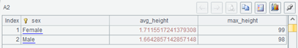
(Because the data is generated randomly, the statistical values will change every time, and they are not in line with common sense. But it does not affect understanding.)
The aggregate operation in the second half of the groups function cannot be written casually. It can only support several aggregate functions made in advance. There are five common aggregate operations: sum, count, avg, max and min. Writing these operations in the parameters is equivalent to executing the aggregate functions for these subsets (also a record sequence).
Aggregation can also be done for an expression, such as:
| A | |
|---|---|
| 1 | … |
| 2 | =A1.groups(sex;min(weight/height/height):min_bmi) |
It is not necessarily to do grouping by field, but also by the result calculated by field.
| A | |
|---|---|
| 1 | =100.new(date(now())-100+~:dt,rand()*100:price) |
| 2 | =A1.select(day@w(dt)>1 && day@w(dt)<7) |
| 3 | =A2.groups(day@w(dt)-1:wday;min(price):min_p,max(price):max_p) |
Group and aggregate the stock data, and calculate the highest and lowest stock prices of all Mondays, Tuesdays,… and Fridays. The calculation results are 5 records (weekends have been excluded).
For the grouping field or expression, we have a term called grouping key. We will understand why we use the word “key” when we’ve learned the later content.
There can also be multiple grouping keys:
| A | |
|---|---|
| 1 | =1000.new(date(now())-1000+~:dt,rand()*100:price) |
| 2 | =A1.select(day@w(dt)>1 && day@w(dt)<7) |
| 3 | =A2.groups(month(dt):m,day@w(dt)-1:wd;avg(price):price) |
A3 can calculate the average stock price on each weekday of each month. When there are multiple grouping expressions, the data table will be split in more detail, and the number of groups will roughly be the same as the product of the number of value types of these grouping keys. For example, the above operation will divide into 12*5=60 groups, because there are 12 types of months and 5 types of weekdays (excluding weekends). The returned table sequence has 60 records.
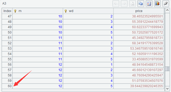
However, this is not absolute. Because in this set of data, there are data on any weekday in any month, these 60 groups will all have corresponding aggregate data. Sometimes the data is incomplete, and some groups will no longer exist. For example, we do a sampling in A2, randomly getting 100 records and then observe the grouping results (we learned how to sample before) to see whether there are always 60 records in the returned table sequence. Please try it yourself.
Because there may be multiple grouping keys, the groups function uses a higher-level semicolon to separate the expression used for grouping keys and the expression used for aggregation in the parameters. Here you can experience the convenience of multi-level parameters.
In fact, group aggregation can also be done without grouping key at all.
| A | |
|---|---|
| 1 | … |
| 2 | =A1.groups(;min(weight/height/height):min_bmi) |
This means that all members are divided into one set, that is, no splitting. For this whole set, calculate some aggregate values, and the returned table sequence has only one record.
However, this operation is not common because it can be done directly with aggregate functions.
Similarly, group aggregation can also have no aggegate value part:
| A | |
|---|---|
| 1 | … |
| 2 | … |
| 3 | =A2.groups(month(dt):m,day@w(dt)-1:wd) |
A3 will calculate the months and weekdays when these stock transactions occur (we can try the results by reducing the amount of data with sampling we just mentioned), that is, we only care about the groups that can be divided, not the aggregate value of each group.
This is a common operation. It will calculate the possible values for grouping keys in a data table and list all the possible values without repetition. The database industry has a special name for this operation, which is called getting the DISTINCT values.
SPL also gives a function id() to calculate DISTINCT.
| A | |
|---|---|
| 1 | … |
| 2 | … |
| 3 | =A2.groups(month(dt):m) |
| 4 | =A2.id(month(dt)) |
Different from the groups()function that returns a table sequence, id() returns a sequence that has no data structure and no field name parameter.
The id() function with multiple parameters does not calculate DISTINCT for multiple grouping keys, but calculates multiple groups of DISTINCT values respectively. If we want to calculate the DISTINCT values for the combined multiple grouping keys, we need to use a sequence expression.
| A | |
|---|---|
| 1 | … |
| 2 | … |
| 3 | =A2.groups(month(dt):m,day@w(dt)-1:wd) |
| 4 | =A2.id(month(dt),day@w(dt)-1) |
| 5 | =A2.id([month(dt),day@w(dt)-1]) |
You can observe the return results of A3, A4 and A5, especially the length of these return values (as table sequence or sequence).
Again, it’s easier to see the difference by sampling the data and then executing these codes.
Now give us some Excel files, and we can already make various classification statistics on the data in them. For example, we have used this data for many times:
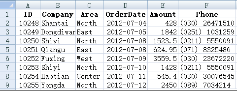
It is very easy to calculate sales amount and order quantity by area or month:
| A | |
|---|---|
| 1 | =T(“data.xlsx”) |
| 2 | =A1.groups(Area;sum(Amount),count(Amount)) |
| 3 | =A2.groups(month@y(OrderDate);sum(Amount),count(Amount)) |
file(…).xlsimport@t()can be simplified into a T() function. Note that SPL is a case sensitive language, and the field names should be written correctly.
It’s easy to calculate the companies that have done business with:
| A | |
|---|---|
| 1 | =T(“data.xlsx”) |
| 2 | =A1.id(Company) |
DISTINCT lets us know that there are groups that do not need to be summarized. In fact, there are groups that should not be summarized.
For example, in a group of people, we want to know who has the same birthday as others. It’s very simple, after grouping by birthday, just see which groups have more than one member. However, the groups() function will force a summary action, and we will lose those divided groups.
Grouping is not always forced to summarize. Sometimes we are also interested in the subset after grouping. In fact, the word grouping has only the meaning of splitting in the dictionary, and does not continue to summarize. Because this operation was invented by SQL, and the set data type of SQL is relatively weak, it is unable to maintain the intermediate results of grouping, so a summary is forced. Over time, the whole industry felt that grouping must be accompanied by summary, and forgot the original intention of grouping.
SPL restores this operation. The group()function without s just group without summary. The s in the name of groups() function means summary.
| A | |
|---|---|
| 1 | =200.new(string(~):ID, date(now())-10000+rand(3000):Birthday) |
| 2 | =A1.group(month(Birthday),day(Birthday)) |
| 3 | =A2.select(~.len()>1).conj() |
Randomly generating the birthdays of 200 people, and then group by birthday (not counting years). The group() function returns the divided groups, that is, a sequence composed of some record sequences, which is equivalent to a two-layer sequence. Then, we just need to see which group has more than one member, and this is the syntax we have learned. Finally, concatenate these groups.
Grouping without summary has practical business significance. Finding someone with the same birthday is just a game. Let’s take another practical example, for the previous Excel file, we want to split it into multiple files according to the Area field for different managers to deal with.
It is reasonable to use grouping operation to split it, but obviously we can’t summarize any more.
| A | B | |
|---|---|---|
| 1 | =T(“data.xlsx”) | =A1.group(Area) |
| 2 | for B1 | >T(A2.Area/“.xlsx”,A2) |
T()function can also write a record sequence directly into an Excel file. After grouping by Area, write each group into a corresponding file. A2.Area is the abbreviation of A2(1).Area. According to the SPL convention, getting a field from a record sequence is equivalent to gettng a field from its first member.
Sometimes, even if we want to get an aggregation result of the grouped subset, it is not easy to calculate, and there is no simple aggregation function to use. In this case, we also need to keep the grouped subsets for further calculation.
For example, we want to group the personnel table by gender, concatenate the names (now some number strings) of people of the same gender into a comma separated string. This is indeed an aggregation result, but SPL does not have such an aggregation function, it can be writen with an expression:
| A | |
|---|---|
| 1 | =100.new(string(~):name,if(rand()<0.5,“Male”,“Female”):sex,50+rand(50):weight,1.5+rand(40)/100:height) |
| 2 | =A1.group(sex).new(~.sex,~.(name).concat@c():Names) |
Just do new() for the subset sequence after grouping.
This operation is common. SPL also allows it to be simplified into the parameters of the group() function:
| A | |
|---|---|
| 1 | … |
| 2 | =A1.group(sex;~.(name).concat@c():Names) |
Note that this is easily confused with groups(). The calculation after the semicolon of group() is equivalent to a simplified new(), and we need to write ~ to represent a grouped subset. But we don’t need to write ~ in groups(). In fact, its calculation method is different. It doesnot calculate the subset first and then calculate the summary value.
As mentioned earlier, there are five common aggregate operations. SPL also provides other aggregate functions that can be used in grouping and aggregation, but most of them do not need to be specifically mentioned. You can check the documents when necessary. There is only one icount() to mention here.
icount(x) returns the number of DISTINCT values of x in each group. This is roughly equivalent to another grouping in the group, but the inner grouping only counts and does not do other summaries.
For example, we want to calculate how many companies each area has done business with:
| A | |
|---|---|
| 1 | =T(“data.xlsx”) |
| 2 | =A1.groups(Area;icount(Company)) |
If you understand the iterative function mentioned earlier, SPL also allows you to spell out new grouping and summary operations. Moreover, after fully understanding the iterative function, you will also realize that groups()and group() use different methods in calculating the summary value. Groups()use the iterative function method to calculate the summary value, and each grouping subset will not be maintained in the process, which will be more efficient and use less memory. This is also the main reason why groups() is designed separately (its syntax is sometimes slightly simpler than group(), but it is only a secondary reason).
In addition, grouping operation is not only valid for structured data, but also for numerical or string sequences.
| A | |
|---|---|
| 1 | =100.(rand(100)).groups(~%2;sum(~)) |
| 2 | =directory(“*.*”).group(filename@e(~)) |
A1 will group integers by parity and calculate the sum of each group; A2 divides the file names under the path into several groups according to the extension.
However, grouping for sequences is relatively uncommon, so we talk about this operation in the structured data section.
SPL Programming - Preface
SPL Programming - 8.5 [Data table] Calculations on the fields
SPL Programming - 9.2 [Grouping] Enumeration and alignment
SPL Official Website 👉 http://www.scudata.com
SPL Feedback and Help 👉 https://www.reddit.com/r/esProc
SPL Learning Material 👉 http://c.scudata.com
SPL Source Code and Package 👉 https://github.com/SPLWare/esProc
Discord 👉 https://discord.gg/ydhVnFH9
Youtube 👉 https://www.youtube.com/@esProc_SPL

