

Multidimensional Analysis Backend Practice 8: Primary-sub Table and Parallel Calculation
Abstract
This series of articles explain how to perform multidimensional analysis (OLAP) in steps with detailed samples. Click to learn more in Multidimensional Analysis Backend Practice 8: Primary-sub Table and Parallel Calculation. Multidimensional Analysis Backend Practice 8: Primary-sub Table and Parallel Calculation
Aim of practice
This issue aims to use ordered merging and integrated storage to implement primary-sub table and perform its parallel multidimensional analysis calculation.
The steps of practice are:
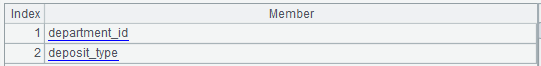
1. Prepare “deposit table”: export the deposit table from the database and generate a primary-sub table along with the customer table as in the following picture:

2. Perform multidimensional analysis calculation on primary-sub table: modify the query code.
3. Perform data updating on primary-sub table.
DEPOSIT_ID NUMBER(20,0), id number of deposit
CUSTOMER_ID NUMBER(10,0), id number of customer
DEPOSIT_DATE DATE, date of deposit
AMOUNT NUMBER(8,2), amount of deposit
DEPARTMENT_ID NUMBER(4,0), id number of department
DEPOSIT_TYPE NUMBER(2,0) type of deposit, range of values 1-5

The multidimensional analysis calculation requirements can be described in the following SQL of Oracle:
select c.department_id,d.deposit_type,sum(d.amount) sum
from customer c left join DEPOSIT d on c.customer_id=d.customer_id
where d.department_id in (10,20,50,60,70,80)
and c.job_id in ('AD_VP','FI_MGR','AC_MGR','SA_MAN','SA_REP')
and d.deposit_date>=to_date('2002-01-01','yyyy-mm-dd')
and d.deposit_date<=to_date('2002-4-31','yyyy-mm-dd')
and c.flag1='1' and c.flag8='1'
group by c.department_id,d.deposit_type
Prepare data
1. Ordered merge
The storage scheme in customer.ctx of previous issues can be directly adopted for the customer table.
The deposit table will be processed in the way of exporting the data in the database to deposit.ctx. And the code sample of etl.dfx is:
A |
B |
|
1 |
=connect@l("oracle") |
=date("2000-01-01") |
2 |
=A1.cursor@d("select * from deposit order by customer_id,deposit_id") |
|
3 |
=A2.new(int(customer_id):customer_id,int(deposit_id):deposit_id,int(interval@m(B1,deposit_date)*100+day(deposit_date)):deposit_date,amount,int(department_id):ddepartment_id,int(deposit_type):deposit_type) |
|
4 |
=file("data/deposit.ctx").create(#customer_id,#deposit_id,deposit_date,amount,department_id,deposit_type;customer_id) |
|
5 |
=A4.append(A3) |
>A4.close(),A1.close() |
A1: connect to the pre-configured oracle database, and @l is used to process the retrieved fields to lowercase. Please note here l is the lowercase L.
B1: define the date as 2000-01-01.
A2: create a cursor based on the database to retrieve the data in “deposit” table. The @d option in the cursor is used to convert “numeric” data in oracle to “double” data rather than “decimal” type of data. “decimal” data have poor performance in java.
A3: use new function to define three calculations.
1. Convert the values that are integers for sure from “double” or “string” to “int”. Use int function to do type conversion directly. But note that “int” can not be greater than 2147483647. The primary key of the sequence number will be the “long” type if the fact table has excessive data than this value.
2. Use “interval” to calculate the different number of months between deposit_date and 2000-01-01, multiply it by 100 and add the day value of deposit_date, then use int to convert the result to an integer and save it as the new deposit_date.
3. department_id is the branch department of deposit, which is the same name as the branch department of account in the customer table, so it needs to be renamed as ddepartment_id.
A4: define a composite table file in columnar storage with the same field names as A3. The parameter customer_id after the semicolon means that the composite table will segment by customer_id field and will not split the records with the same customer_id value to two segments when appending data, which prepares to retrieve data by segment in parallel.
A5: calculate the A3 cursor while exporting to the composite table file.
B5: close the composite table file and the database connection.
The size of the exported file deposit.ctx is 4.2G.
2. Integrated storage
Modify etl.dfx to store the customer data and deposit data as fact table and attached table in the composite table file. The code is as follows:
A |
B |
|
1 |
=connect@l("oracle") |
=date("2000-01-01") |
2 |
=A1.cursor@d("select * from customer order by customer_id") |
|
3 |
=A1.cursor@d("select * from deposit order by customer_id,deposit_id") |
|
4 |
=A1.query@d("select job_id from jobs order by job_id") |
=file("data/2job.btx").export@z(A4) |
5 |
=A4.(job_id) |
|
6 |
=A2.new(int(customer_id):customer_id,int(department_id):department_id,A5.pos@b(job_id):job_num,int(employee_id):employee_id,int(interval@m(B1,begin_date)*100+day(begin_date)):begin_date,first_name,last_name,phone_number,job_title,float(balance):balance,department_name,int(flag1):flag1,int(flag2):flag2,int(flag3):flag3,int(flag4):flag4,int(flag5):flag5,int(flag6):flag6,int(flag7):flag7,int(flag8):flag8,int(vip_id):vip_id,int(credit_grade):credit_grade) |
|
7 |
=A3.new(int(customer_id):customer_id,int(deposit_id):deposit_id,int(interval@m(B1,deposit_date)*100+day(deposit_date)):deposit_date,amount,int(department_id):ddepartment_id,int(deposit_type):deposit_type) |
|
8 |
=file("data/customer_deposit.ctx").create@y(#customer_id,department_id,job_num,employee_id,begin_date,first_name,last_name,phone_number,job_title,balance,department_name,flag1,flag2,flag3,flag4,flag5,flag6,flag7,flag8,vip_id,credit_grade) |
|
9 |
=A8.append(A6) |
=A8.attach(deposit,#deposit_id,deposit_date,amount,ddepartment_id,deposit_type) |
10 |
=B9.append(A7) |
|
11 |
=A8.close() |
|
A1: connect to the pre-configured oracle database.
B1: define the date as 2000-01-01.
A2, A3: create a cursor based on the database to retrieve the data in “customer table” and “deposit” table.
A4, B4, A5: retrieve “jobs” data from the database for data conversion in “customer”.
A6, A7: define the data conversion on two cursors.
A9: define “customer” composite table file. A10: retrieve the “customer” data from the database cursor and write them in composite table, which is called fact table.
B9: add an attached table “deposit” to the composite table file, the first primary key customer_id is the same as the primary key of fact table, so it will be omitted. Other fields should not have the same name as those in fact table.
B10: retrieve data from the database cursor and write them into attached table.
A11: close the composite table and the database connection.
The size of the exported file customer_deposit.ctx is 7.4G.
Multidimensional analysis calculation
1. Ordered merge
The SPL code consists of olapJoinx.dfx and customerJoinx.dfx, the former is the entry of calling and the given parameters are arg_table and arg_json, the latter is used to parse arg_json.
The value of arg_table is customerJoinx.
The value of arg_json is:
{
       aggregate:
              [
                     {
                            func:"sum",
                            field:"amount",
                            alias:"sum"
                     }
              ],
       group:
              [
                     "department_id",
                     "deposit_type"
              ],
       slice:
              [
                     {
                            dim:"ddepartment_id",
                            value:[10,20,50,60,70,80]
                     },
                     {
                            dim:"job_id",
                      value:["AD_VP","FI_MGR","AC_MGR","SA_MAN","SA_REP"]
                     },
                     {
                            dim:"deposit_date",
                            interval:[date("2002-01-01"),date("2020-12-31")]
                     },
                     {
                            dim:"flag1",
                            value:"1"
                     },
                     {
                            dim:"flag8",
                            value:"1"
                     }
              ]
}
The code of customerJoinx.dfx is:
A |
B |
C |
|
1 |
func |
||
2 |
if A1.value==null |
return "between("/A1.dim/","/A1.interval(1)/":"/A1.interval(2)/")" |
|
3 |
else if ifa(A1.value) |
return string(A1.value)/".contain("/A1.dim/")" |
|
4 |
else if ifstring(A1.value) |
return A1.dim/"==\""/A1.value/"\"" |
|
5 |
else |
return A1.dim/"=="/A1.value |
|
6 |
func |
||
7 |
if ifa(A6) |
return A6.(if(A9.pos(~),"c."/~,"d."/~)) |
|
8 |
else |
return if(A9.pos(A6),"c."/A6,"d."/A6) |
|
9 |
="customer_id,department_id,job_num,employee_id,begin_date,first_name,last_name,phone_number,job_title,balance,department_name,flag1,flag2,flag3,flag4,flag5,flag6,flag7,flag8,vip_id,credit_grade".split@c() |
||
10 |
=json(arg_json) |
=date("2000-01-01") |
|
11 |
=func(A6,A10.aggregate.(field)) |
=A10.aggregate.(~.func/"("/A11(#)/"):"/~.alias).concat@c() |
|
12 |
=A10.group.(if(~=="job_id","job_num",~)) |
||
13 |
=A12.(if(~=="begin_yearmonth","begin_date\\100:begin_yearmonth",~)) |
=func(A6,A13).concat@c() |
|
15 |
=[] |
=[] |
|
16 |
for A10.slice |
if (A15.dim=="begin_date"|| A15.dim=="deposit_date") && A15.value!=null |
>A15.value=int(interval@m(C10,eval(A15.value))*100+day(eval(A15.value))) |
17 |
else if (A15.dim=="begin_date"|| A15.dim=="deposit_date") && A15.value==null |
=A15.interval.(~=int(interval@m(C10,eval(~))*100+day(eval(~)))) |
|
18 |
else if A15.dim=="job_id" |
>A15.dim="job_num" |
|
19 |
>A15.value=A15.value.(job.pos@b(~)) |
||
20 |
else if like(A15.dim, "flag?") |
>A15.value=int(A15.value) |
|
21 |
>B14|=A15.dim |
=A15.dim=func(A6,A15.dim) |
|
22 |
=[func(A1,A15)] |
>A14|=B21 |
|
23 |
=A10.aggregate.(field) |
=A12.(if(~=="begin_yearmonth","begin_date",~)) |
|
24 |
=(A22|B14|C22|["customer_id"]).id() |
=A23^A9 |
=A23\B23|["customer_id"] |
25 |
=A10.group|A10.aggregate.(alias) |
=A24(A24.pos("job_id"))="job(job_num):job_id" |
|
26 |
=A24(A24.pos("begin_yearmonth"))="month@y(elapse@m(date(\""/C10/"\"),begin_yearmonth)):begin_yearmonth" |
||
27 |
=A24(A24.pos("begin_date"))="elapse@m(B4,begin_date\\100)+(begin_date%100-1):begin_date" |
||
28 |
return B23.concat@c(),C23.concat@c(),B11,C13,A14.concat("&&"),A24.concat@c() |
||
Area from A1 to C8 is subprogram which only executes when being called. We will explain them in the order of execution for the sake of better illustration.
A9: list the fields of “customer” table to identify which table the parameters in arg_json belongs to.
A10: parse arg_json to a table sequence and the return result is a nested multi-layer table sequence as follows:

The “aggregate” in it is:

The “group” is:
The “slice” is:

C10: define the beginning date as 2000-01-01 for the conversion of date values in parameters and results.
A11: call the subprogram A6, and pass the “field” sequence A10.aggregate.(field) of aggregate expression to A6 as a parameter.
B7: if the given parameter is a sequence, then C7 identifies whether each of the sequence member belongs to the “customer” table, and adds the “c.” prefix if the member does, otherwise adds the “d.” prefix. Return C7.
B8: if the given parameter is not a sequence, it directly identifies whether A6 belongs to the “customer” table, and adds the “c.” prefix if A6 does, otherwise adds the “d.” prefix. Return C8.
At this point subprogram A6 returns:

B11: first calculate the aggregate expression and the corresponding member of A11 as a colon-concatenated string sequence as follows:

Then concatenate the sequence as a string with a comma: sum(d.amount):sum, i.e., the aggregate expression.
A12: replace the job_id in “group” with job_num.
A13: replace the begin_yearmonth in A12 with expression begin_date\100:begin_yearmonth.
B13: concatenate the members of A13 as a string with commas: c.department_id,d.deposit_type, i.e., the grouping expression.
A14: define an empty sequence which prepares to store slice (filtering conditions) expression sequence.
B14: define an empty sequence which prepares to store the field names required for slice(filtering conditions).
A15: loop through A10.slice, and the loop body is B15 to C21 in which from B15 to C20 is the optimization conversion to the “value” or “interval” of “slice”.
B15: if the “dim” of current “slice” is begin_date and the “value” is not null, that is, the begin_date equals to the specified date. For example, begin_date==date("2010-11-01"). In this case, C15 calculates the converted integer value of date("2010-11-01") and assigns it to the “value” of A15.
B16: if the “dim” is begin_date and the “value” is null, that is, the begin_date is between two dates. For example: begin_date is between date("2002-01-01") and date("2020-12-31"). In this case, C16 calculates the converted integer values of those two dates and assigns them to two members of “interval” in A15.
B17: if the “dim” is job_id, that is, job_id is an enumeration value, for example, ["AD_VP","FI_MGR","AC_MGR","SA_MAN","SA_REP"].contain(job_id). In this case, C17 converts the “dim” of A15 to job_num and C18 converts the enumeration value “value” of A15 to the position in the sequence of global variable “job”, i.e., job_num integer sequence. For example: [5,7,2,15,16].
B19: if the “dim” is flag1, flag2, ..., flag8, that is, the flag bit equals to “1” or “0”. In this case, C18 converts the “value” of A15 from strings to integers.
B20: append A15.dim to B14.
C20: use A15.dim as parameter to call subprogram A6, add table name prefix to the field name, and assign the return result to A15.dim. The execution result is:

B21: take the result of B15 to C20, which converts the “value” or “interval” of “slice” for performance optimization, as parameter to call subprogram A1. Subprogram A1 is identical to the A1 code in the second article.
C21: append the return result of func A1 to A14. Continue the loop in A15 until it is over. And the sequence of slice expressions is well prepared.
A22: get the “field” in “aggregate”, that is, all the field names used in the aggregate expression.
C22: replace begin_yearmonth in “group” with begin_date, and the result is all the field names used in the grouping expression.
A23: add a “customer_id” after concatenating A22, B21, and C22, then remove the duplicates:

B23: calculate the intersection of the members in A23 and A9, i.e., the fields of “customer” table.
C23: calculate the members after A23 removes B23, i.e., the fields of “deposit” table.
A24: prepare the conversion expression of result set display value from here. Concatenate A10.group with A10.aggregate.alias sequence as follows:

C24: replace the job_id in A24 with conversion statement which is used to convert the job_num in result set to job_id.
A25: replace the begin_yearmonth in A24 with conversion statement which is used to convert the begin_yearmonth in grouping fields from integers to yyyymm.
A26: replace the begin_date in A24 with conversion statement which is used to convert the integer date values in grouping fields to date type. At this point A24 is the prepared result set display value conversion expression:

A27: return B23.concat@c(), C23.concat@c(), B11, C13, A14.concat("&&"), and A24.concat@c() respectively as:
The field names of “customer” table used in the calculation: customer_id, department_id, flag1, flag8,job_num
The field names of “deposit” table used in the calculation: amount, ddepartment_id, deposit_date, deposit_type, customer_id
The aggregate expression: sum(d.amount):sum
The grouping expression: c.department_id,d.deposit_type
The slice expression:
[10,20,50,60,70,80].contain(d.ddepartment_id) && [5,7,2,15,16].contain(c.job_num) && between(d.deposit_date,2401:25131) && c.flag1==1 && c.flag8==1
The result set display value conversion expression:
department_id,deposit_type,sum
The value of parameter arg_table of the front-end calling entry olapJoinx.dfx is customerJoinx.dfx, and the code is:
A |
|
1 |
=call(arg_table/".dfx",arg_json) |
2 |
=file("data/customer.ctx").open().cursor@m(${A1(1)};;2) |
3 |
=file("data/deposit.ctx").open().cursor(${A1(2)};;A2) |
4 |
=joinx(A2:c,customer_id; A3:d,customer_id) |
5 |
=A4.select(${A1(5)} ) |
6 |
return A5.groups(${A1(4)};${A1(3)}).new(${A1(6)}) |
A2: the code actually executed is: =file("data/customer.ctx").open().cursor@m(customer_id,department_id,flag1,flag8,job_num;;2), which is used to create a cursor on the file and set the field names that need to be retrieved for cursor filtering, and the number of parallel threads is 2.
A3: the code actually executed is: =file("data/deposit.ctx").open().cursor(amount,ddepartment_id,deposit_date,deposit_type,customer_id;;A2)
Get the multi-cursor of deposit according to the value of multi-cursor A2, and the paths of cursor is also 2.
A4: orderly merge the two multi-cursors, and the associate field is customer_id.
A5: the code actually executed is: =A4.select([10,20,50,60,70,80].contain(d.ddepartment_id) && [5,7,2,15,16].contain(c.job_num) && between(d.deposit_date,2401:25131) && c.flag1==1 && c.flag8==1 )
Define conditional filtering calculation on the merged cursors.
A6: the code actually executed is: return A5.groups(c.department_id,d.deposit_type; sum(d.amount):sum).new(department_id,deposit_type,sum)
Define grouping and aggregation on the cursors and execute the calculation defined by the cursors.
The Java code used to call the SPL code remains unchanged compared to last issue as long as the calling parameters are adjusted.
2. Integrated storage of primary-sub table
The SPL code consists of olap.dfx and customer_deposit.dfx, the former is the entry of calling and the given parameters are arg_table and arg_json, the latter is used to parse arg_json.
The value of arg_table is customer_deposit.
The value of arg_json is the same as that of ordered merge.
The code of customer_deposit.dfx is:
A |
B |
C |
|
1 |
func |
||
2 |
if A1.value==null |
return "between("/A1.dim/","/A1.interval(1)/":"/A1.interval(2)/")" |
|
3 |
else if ifa(A1.value) |
return string(A1.value)/".contain("/A1.dim/")" |
|
4 |
else if ifstring(A1.value) |
return A1.dim/"==\""/A1.value/"\"" |
|
5 |
else |
return A1.dim/"=="/A1.value |
|
6 |
=json(arg_json) |
=date("2000-01-01") |
|
7 |
=A6.aggregate.(~.func/"("/~.field/"):"/~.alias).concat@c() |
||
8 |
=A6.group.(if(~=="job_id","job_num",~)) |
||
9 |
=A8.(if(~=="begin_yearmonth","begin_date\\100:begin_yearmonth",~)).concat@c() |
||
10 |
=A6.aggregate.(field) |
=A8.(if(~=="begin_yearmonth","begin_date",~)) |
|
11 |
=(A10|C10).id().concat@c() |
||
13 |
=[] |
||
14 |
for A6.slice |
if (A13.dim=="begin_date"||A13.dim=="deposit_date") && A13.value!=null |
>A13.value=int(interval@m(C6,eval(A13.value))*100+day(eval(A13.value))) |
15 |
else if (A13.dim=="begin_date"||A13.dim=="deposit_date") && A13.value==null |
=A13.interval.(~=int(interval@m(C6,eval(~))*100+day(eval(~)))) |
|
16 |
else if A13.dim=="job_id" |
>A13.dim="job_num" |
|
17 |
>A13.value=A13.value.(job.pos@b(~)) |
||
18 |
else if like(A13.dim, "flag?") |
>A13.value=int(A13.value) |
|
19 |
=[func(A1,A13)] |
>A12|=B18 |
|
20 |
=A6.group|A6.aggregate.(alias) |
=A19(A19.pos("job_id"))="job(job_num):job_id" |
|
21 |
=A19(A19.pos("begin_yearmonth"))="month@y(elapse@m(date(\""/C6/"\"),begin_yearmonth)):begin_yearmonth" |
||
22 |
=A19(A19.pos("begin_date"))="elapse@m(B4,begin_date\\100)+(begin_date%100-1):begin_date" |
||
23 |
return A11,A7,A9,A12.concat("&&"),A19.concat@c() |
||
As we can see, the code is basically the same as customer.ctx in the third issue except for the addition of processing deposit_date in B14 and B15.
Modify olap.dfx to calculate the fact table and attached table using integrated storage, and the code is:
A |
B |
|
1 |
=call(arg_table/".dfx",arg_json) |
=file("data/"/arg_table/".ctx").open() |
2 |
=arg_table.split("_") |
|
3 |
if A2.len()==2 |
=B1.attach(${A2(2)}) |
4 |
=B3.cursor@m(${A1(1)};${A1(4)};2) |
return A4.groups(${A1(3)};${A1(2)}).new(${A1(6)}) |
A1: call customer_deposit.dfx.
B2: open composite table file data/customer_deposit.ctx.
A2: separate the arg_table parameter values with underscores, and the results are:

The first member is the name of fact table and the second is the name of attached table.
A3: if the length of A2 is 2, then B3 opens the attached table, and the name will be the second member of A2, i.e., “deposit”.
A4: the code actually executed is: =A3.cursor@m(amount,department_id,deposit_type;[10,20,50,60,70,80].contain(ddepartment_id) && [5,7,2,15,16].contain(job_num) && between(deposit_date,2401:25131) && flag1==1 && flag8==1)
B4: the code actually executed is: return A4.groups(department_id,deposit_type; sum(amount):sum).new(department_id,deposit_type,sum)
The Java code used to call the SPL code remains unchanged compared to last issue as long as the calling parameters are adjusted.
The total execution time of Java code plus the backend calculation of return results is as follows:
Calculation method |
Single-thread |
Two-thread |
Note |
Ordered merge |
136 seconds |
86 seconds |
|
Integrated storage |
62 seconds |
41 seconds |
As can be seen from the above comparison, integrated storage can improve the calculation performance compared to ordered merge, and it is also compatible with the code for single wide table OLAP calculations.
New added data
Similar to the customer table, deposit table also has new added data every day which need to be added to composite table file regularly. We can modify etlAppend.dfx, and the cellset parameter is:

The SPL code is:
A |
B |
|
1 |
=connect@l("oracle") |
|
2 |
=A1.query@d("select c.customer_id customer_id,c.department_id department_id,job_id ,employee_id , begin_date, first_name, last_name, phone_number, job_title, balance, department_name, flag1, flag2, flag3, flag4, flag5, flag6, flag7, flag8, vip_id , credit_grade, deposit_id ,deposit_date ,amount,d.department_id ddepartment_id,deposit_type from customer c left join DEPOSIT d on c.customer_id=d.customer_id where begin_date=? order by c.customer_id,deposit_id",today) |
|
3 |
=A1.query@d("select job_id from jobs order by job_id") |
|
4 |
=A3.(job_id) |
=date("2000-01-01") |
5 |
=A2.new(int(customer_id):customer_id,int(department_id):department_id,A4.pos@b(job_id):job_num,int(employee_id):employee_id,int(interval@m(B4,begin_date)*100+day(begin_date)):begin_date,first_name,last_name,phone_number,job_title,float(balance):balance,department_name,int(flag1):flag1,int(flag2):flag2,int(flag3):flag3,int(flag4):flag4,int(flag5):flag5,int(flag6):flag6,int(flag7):flag7,int(flag8):flag8,int(vip_id):vip_id,int(credit_grade):credit_grade,int(deposit_id):deposit_id,int(interval@m(B4,deposit_date)*100+day(deposit_date)):deposit_date,amount,int(ddepartment_id):ddepartment,int(deposit_type):deposit_type) |
|
6 |
=A5.groups(customer_id,department_id,job_num ,employee_id , begin_date, first_name, last_name, phone_number, job_title, balance, department_name, flag1, flag2, flag3, flag4, flag5, flag6, flag7, flag8, vip_id , credit_grade) |
|
7 |
=A5.new(customer_id,deposit_id ,deposit_date ,amount,ddepartment_id,deposit_type) |
|
8 |
=file("data/customer_deposit.ctx").open() |
=A8.append(A6.cursor()) |
9 |
=A8.attach(deposit) |
=A9.append(A7.cursor()) |
10 |
>A8.close(),A1.close() |
|
A1: connect to oracle database.
A2: retrieve the customer data and deposit data of the current day based on begin_date.
A3: retrieve the data of “jobs” table for data type conversion.
A4: retrieve the sequence of job_id. B5: define the beginning date.
A5: define the conversion calculation on data type.
A6: retrieve the customer data in it.
A7: retrieve the deposit data in it.
A8: open customer_deposit.ctx. B6: append the data of A6.
A9: open the attached table “deposit”. B9: append the data of B9.
A10: close the file and the database connection.
etlAppend.dfx needs to be executed regularly every day, which is done by using ETL tools or OS timed tasks to invoke the esProc script from the command line.
For example:
C:\Program Files\raqsoft\esProc\bin>esprocx d:\olap\etlAppend.dfx
SPL Official Website 👉 http://www.scudata.com
SPL Feedback and Help 👉 https://www.reddit.com/r/esProc
SPL Learning Material 👉 http://c.scudata.com
SPL Source Code and Package 👉 https://github.com/SPLWare/esProc
Discord 👉 https://discord.gg/ydhVnFH9
Youtube 👉 https://www.youtube.com/@esProc_SPL


Chinese version