1. Storage scheme

Bin file adopts the row-based storage, whilst composite table has two storage schemes, columnar and row-based. Both schemes will compress the data to some extent.

 

First of all, we create an ordinary text file and generate some data in it. The code sample is:

	A	B
1	=file("txt/employee.txt")
2	=file("info/ming_en_female.txt").import@i()	=A2.len()
3	=file("info/ming_en_male.txt").import@i()	=A3.len()
4	=file("info/xing_en.txt").import@i()	=A4.len()
5	=city=file("info/city_en.txt").import@i()	=A5.len()
6	=salary=20000	/10000~30000
7	=["one","two","three","four","five","six","seven","eight","nine","ten"]	=A7.len()
8	=height=50	/160~210cm
9	=weight=50	/50~100kg
10	=birthtime=946656	/1970~2000
11	for 100	=to((A11-1)*100000+1,A11*100000).new(~:id,if(rand(2)==0,A2(rand(B2)+1),A3(rand(B3)+1))+" "+A4(rand(B4)+1):name,if(A2.pos(name.array(" ")(1)),"Female","Male"):sex,A5(rand(B5-1)+1):city,date(rand(birthtime)*long(1000000)):birthday,rand(salary)+10000:salary,A7(rand(B7-1)+1):level,rand(height)+160:height,rand(weight)+50:weight,if(rand(2)==0,A2(rand(B2)+1),A3(rand(B3)+1))+"&"+A4(rand(B4)+1)+"  Co. Ltd":company)
12		=A1.export@at(B11)

[Code 1.1]

 

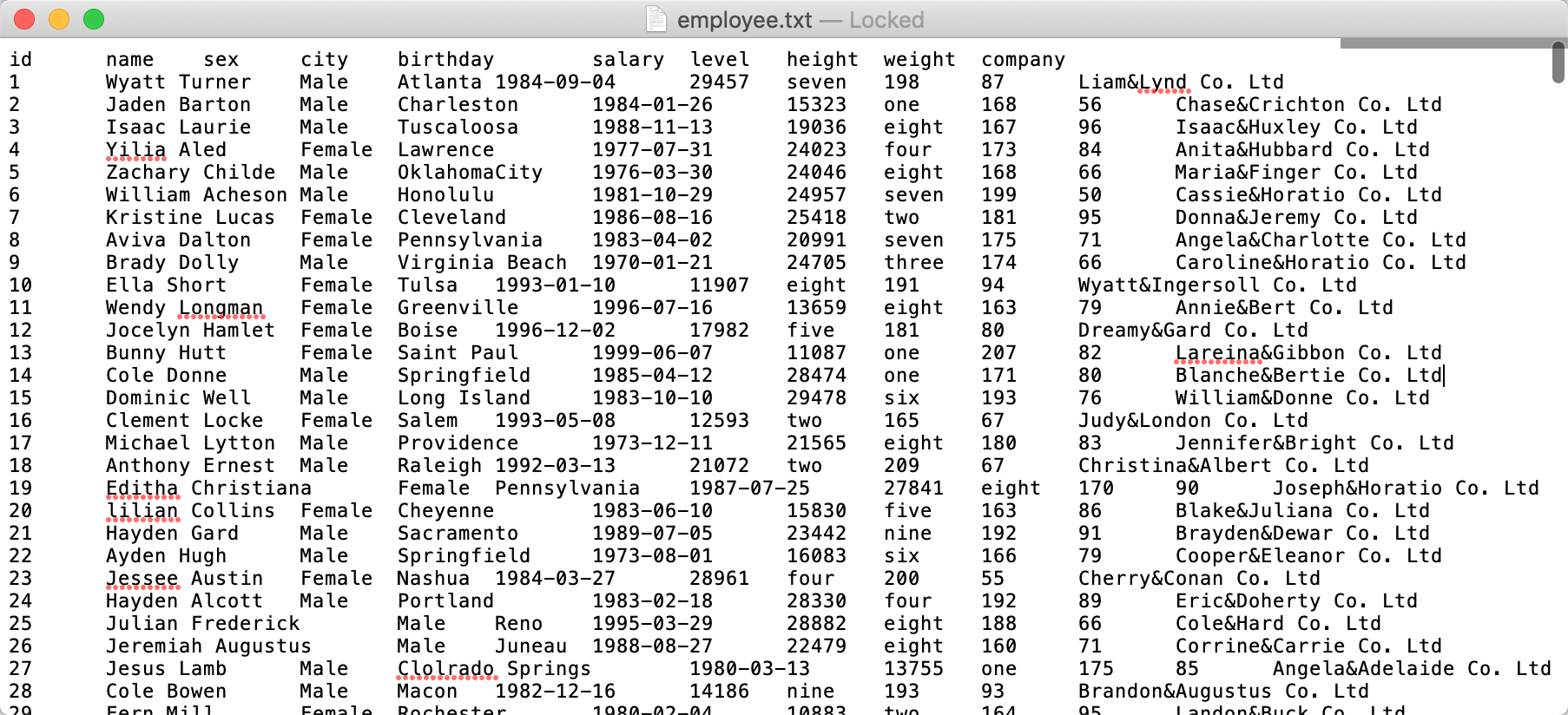
Code 1.1 is to create a txt file with 10 million records in total. And some of the data are shown in Figure 1.1:

[Figure 1.1]

 

	A
1	=file("txt/employee.txt").cursor@t()
2	=file("btx/employee.btx").export@ab(A1)

[Code 1.2]

 

	A
1	=file("txt/employee.txt").cursor@t()
2	=file("ctx/employee.ctx").create(#id,name,sex,city,birthday,salary,level,height,weight,company).append(A1)

[Code 1.3]

 

	A
1	=file("txt/employee.txt").cursor@t()
2	=file("ctx/employee@r.ctx").create@r(#id,name,sex,city,birthday,salary,level,height,weight,company).append(A1)

[Code 1.4]

 

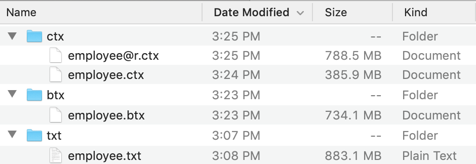
Code 1.2, Code 1.3 and Code 1.4 convert the txt file created in Code 1.1 to bin file employee.btx, composite table file of columnar storage employee.ctx and composite table of row-based storage employee@r.ctx respectively. The file sizes are shown in Figure 1.2.

[Figure 1.2]

 

According to the hard disk space they occupy, we can sort them as txt > row-based composite table > bin file > columnar composite table in descending order. It is obvious that, with different file storage scheme, the same data occupy different hard disk space, which will further lead to various traversal efficiency directly.

 

By placing the fields with a large number of duplicates in the front, the sorting operation can improve the efficiency of data compression in columnar composite table significantly.

 

***Here the example is not correct because we ought to put the sorted fields in the front.

 

	A
1	=file("ctx/employee.ctx").open().cursor().sortx(level,height,weight,city)
2	=file("ctx/employee_sort.ctx").create(#id,name,sex,city,birthday,salary,level,height,weight,company).append(A1)

[Code 1.5]

 

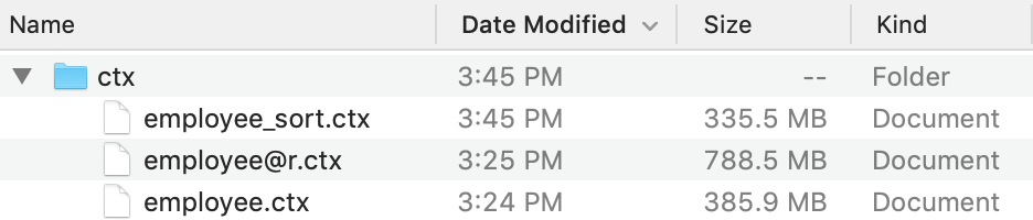
Code 1.5 is to sort the level, height, weight, and city columns of the original composite table file in order.

 

The sorted composite table file employee_sort.ctx is obviously smaller than the original file employee.ctx, as shown in Figure 1.3.

 

[Figure 1.3]

 

2. Parallel traverse

The select@m function can be used to perform parallel calculation when filtering the table sequence.

	A
1	=now()
2	=file("ctx/employee.ctx").open().cursor(;level=="two" && city=="Reno").fetch()
3	=interval@ms(A1,now())
4	=now()
5	=file("ctx/employee.ctx").open().cursor@m(;level=="two" && city=="Reno";4).fetch()
6	=interval@ms(A4,now())
7	=file("ctx/employee.ctx").opene().cursor().fetch()
8	=now()
9	=A7.select(level=="two" && city=="Reno")
10	=interval@ms(A8,now())
11	=now()
12	=A7.select@m(level=="two" && city=="Reno")
13	=interval@ms(A11,now())

[Code 2.1]

 

In Code 2.1:

A2 and A5 are the results of serial and parallel operation on external storage respectively, taking 2,742 and 828 milliseconds.

 

A9 and A112 are the result of serial and parallel operation in memory respectively, taking 1,162 and 470 milliseconds.

 

We can define multi-cursor on both bin file and composite table to perform parallel traversing. But the multi-cursor may not execute very fast in the case of columnar storage + mechanical hard disk + too many fetched columns.

	A
1	=now()
2	=file("btx/employee@z.btx").cursor@bm(;4).select(level=="two" && city=="Reno").fetch()
3	=interval@ms(A1,now())
4	=now()
5	=file("ctx/employee.ctx")
6	=A5.open().cursor@m(;;4).select(level=="two" && city=="Reno")
7	=A6.fetch()
8	=interval@ms(A4,now())

[Code 2.2]

 

In Code 2.2:

The first three lines are the parallel traversing on the bin file, taking 1,861 milliseconds.

 

The last five lines are the multi-cursor parallel traversing on the columnar composite table with the same data, which takes 2,282 milliseconds.

 

When performing parallel with the fork statement, do not return cursor. A cursor is just a definition, while it does not perform actual data fetching. So this kind of parallel is meaningless, and only the parallel calculation which performs actual data fetching actions such as “fetch” or “groups” in the fork code block does make sense.

	A	B
1	=file("ctx/employee.ctx").open()
2	=now()
3	fork to(4)	=A1.cursor(;level=="one" &&  height==180;A3:4).fetch()
4		return B3
5	=A3.conj()
6	=interval@ms(A2,now())
7	=file("ctx/employee.ctx").open()
8	=now()
9	fork to(4)	=A7.cursor(;level=="one" && height==180;A9:4)
10		return B9
11	=A9.conjx().fetch()
12	=interval@ms(A8,now())

[Code 2.3]

 

In Code 2.3, the first six lines are to fetch data in fork code block and then union the results, which costs 865 milliseconds. Form the seventh line to the twelfth line, after the fork function returns the cursor, merge the results and then perform “fetch”, which takes 1,709 milliseconds in total.

 

3. Filtering condition

When there are multiple conditions &&, the writing position is very important. If the sub-clause in the front is false, other behind clauses won’t be calculated. So if we write those conditions that are easy to be false in the front, the calculations on later conditions will decrease in number.

	A
1	=file("btx/employee.btx").cursor@b().fetch()
2	=now()
3	=A1.select(salary < 10010 && like(name,"*d*"))
4	=interval@ms(A2,now())
5	=now()
6	=A1.select(like(name,"*d*") && salary < 10010)
7	=interval@ms(A5,now())

[Code 3.1]

 

In Code 3.1:

The condition in A3 is salary < 10010 && like(name,"*d*"), and the sub-clause in the front returns a relatively small result set, which costs 748 milliseconds in total.

 

The condition in A6 is like(name,"*d*") && salary < 10010, and the sub-clause in the front returns a relatively big result set, which costs 1,814 milliseconds in total.

 

When searching members in s set (IN judgment), we should avoid calculating the set in the filtering condition temporarily. Instead, we should first sort the members and then use pos@b or contain@b to make judgment, which will use the binary search.

 

	A
1	=100.(rand(1000000)+1)
2	=file("txt/keys.txt").export(A1)

[Code 3.2]

 

In Code 3.2:

A1: Take 100 random numbers ranging from 1 to 1,000,000.

 

A2: Store these 100 randoms numbers in keys.txt file to ensure consistent data for subsequent tests.

 

	A
1	=file("txt/keys.txt").import@i()
2	=A1.(~*10)
3	=file("ctx/employee.ctx").open()
4	=now()
5	=A3.cursor(;A2.pos(id)).fetch()
6	=interval@ms(A4,now())

[Code 3.3]

 

In Code 3.3:

A2: Multiply each of the pre-prepared key value by 10.

 

A5: Use the pos function to find and retrieve the members that satisfy A2 in the composite table file employee.ctx, which takes 15,060 milliseconds.

 

	A
1	=file("txt/keys.txt").import@i()
2	=file("ctx/employee.ctx").open()
3	=now()
4	=A2.cursor(;A1.(~*10).pos(id)).fetch()
5	=interval@ms(A3,now())

[Code 3.4]

 

In Code 3.4:

We move the set in A2 of Code 3.3 to the cursor filtering condition in A4 of Code 3.4 to calculate the set temporarily, and the execution time is 32,105 milliseconds. The operation takes twice as much time compared with Code 3.3. Therefore, it should still be avoided even though we can get the same result.

 

	A
1	=file("txt/keys.txt").import@i()
2	=A1.(~*10).sort()
3	=file("ctx/employee.ctx").open()
4	=now()
5	=A3.cursor(;A2.pos@b(id)).fetch()
6	=interval@ms(A4,now())

[Code 3.5]

 

We can further optimize Code 3.5 based on Code 3.3.

 

Sort A2 of Code 3.3 to get the ordered key values.

 

Option @b is used on the pos function in A5 to perform the binary search. And the execution time is 7,854 milliseconds, which is nearly twice faster than the operation in Code 3.3.

 

switch@i@d can be used to achieve quick key value filtering, and hash index is usually more efficient than binary search.

 

	A
1	=file("txt/keys.txt").import@i()
2	=A1.(~*10).sort()
3	=file("ctx/employee.ctx").open()
4	=now()
5	=A3.cursor().switch@i(id,A2).fetch()
6	=interval@ms(A4,now())

[Code 3.6]

 

In Code 3.6:

A5: switch@i is used to filter out the data satisfying sequence A2, and the result stays the same with Code 3.3, Code 3.4 and Code 3.5, costing 7,104 milliseconds. The switch function can automatically create index. @d option can also achieve the filtering, which will not be explained with a separate example here.

 

4. Filtering in advance

We can write some filtering conditions when the composite table cursor is being created. And esProc will identify these conditions and use the sorting information of the composite table itself to quickly jump to the corresponding data location. In addition, the retrieved fields will not be read if these conditions are not satisfied, thus decreasing the number of object generation. But these effects will no longer exist if we first generate the cursor and then do the filtering. Here is an example:

 

	A
1	=file("ctx/employee.ctx").open()
2	=now()
3	=A1.cursor(city,sex;level=="one" && height<180)
4	=A3.groups(city;count(sex=="Male"):Male,count(sex=="Female"):Female)
5	=interval@ms(A2,now())
6	=now()
7	=A1.cursor().select(level=="one" && height<180)
8	=A7.groups(city;count(sex=="Male"):Male,count(sex=="Female"):Female)
9	=interval@ms(A6,now())

[Code 4.1]

 

In Code 4.1:

A3 is to write filtering condition level=="one" && height<180 when the composite table cursor is being created, and retrieve only two columns of data, respectively city and sex.

 

A7 is to filter the data with the filtering condition in select function after the composite table cursor is created.

 

Then the same grouping and aggregation operations are performed on both of them, and the former takes 1,206 milliseconds whereas the latter takes 4,740 milliseconds.

 

5. Fetching from cursor

The performance of fetching data from cursor is related to the number of records fetched each time. Here we do some tests with tens of thousands of rows rather than retrieving one row at a time.

 

	A	B
1	=file("ctx/employee.ctx").open().cursor()
2	>ctx_length_10=0
3	=now()
4	for A1,10	=A4.len()
5		>ctx_length_10=ctx_length_10+B4
6	=interval@ms(A3,now())
7	=file("ctx/employee.ctx").open().cursor()
8	>ctx_length_50000=0
9	=now()
10	for A7,50000	=A10.len()
11		>ctx_length_50000=ctx_length_50000+B10
12	=interval@ms(A9,now())

[Code 5.1]

 

In Code 5.1:

The code traverses the composite table cursor to get the result, and cumulate the number of records of each result.

 

In the first 6 lines, the traversing operation fetches 10 records each time, and the final execution time is 7,823 milliseconds.

 

In the last 6 lines, the traversing operation fetches 50,000 records each time, and the finial execution time is 3,923 milliseconds.

 

The skip function can be used to count the number, so we don’t have to load the cursor data to generate java objects.

 

	A
1	=file("ctx/employee.ctx").open()
2	=now()
3	=A1.cursor(#1;).fetch().len()
4	=interval@ms(A2,now())
5	=now()
6	=A1.cursor().skip()
7	=interval@ms(A5,now())

[Code 5.2]

 

In Code 5.2:

A3 is to retrieve the first column when the composite table cursor is created, and then get its length.

 

A6 is to use skip function on the composite table cursor to get the number of records of the composite table.

 

The above mentioned cells both return a value of 10,000,000 after calculation, but the former takes 9,676 milliseconds and the latter takes 6,473 milliseconds.

 

6. Multi-purpose traverse

With the channel technique, we can get multiple results from the same one traversal to decrease the hard disk access.

 

	A	B	C
1	=file("ctx/employee.ctx").create().cursor()
2	=channel(A1)	=channel(A1)	=channel(A1)
3	>A2.select(salary<10123 && level=="nine").fetch()	>B2.select(level=="two" && height==183).fetch()	>C2.select(city=="Reno" && weight>95).fetch()
4	=now()
5	for A1,100000
6	=A2.result()	=B2.result()	=C2.result()
7	=interval@ms(A4,now())
8	=now()
9	=file("ctx/employee.ctx").create().cursor().select(salary<10123 && level=="nine").fetch()	=file("ctx/employee.ctx").create().cursor().select(level=="two" && height==183).fetch()	=file("ctx/employee.ctx").create().cursor().select(city=="Reno" && weight>95).fetch()
10	=interval@ms(A8,now())

[Code 6.1]

 

In Code 6.1:

A2, B2 and C2 are respectively the channels created on the composite table cursor A1. A3, B3 and C3 define various filtering conditions and data fetching on the three channels. A6 traverses the composite table cursor and fetches 100,000 records each time. A6, B6 and C6 get the result sets returned by the filtering conditions defined previously. And the total execution time is 5,182 milliseconds.

 

The three cells in the ninth line does not use the channel technique, instead, they respectively create the composite table cursors and then get the results returned by the three same filtering conditions defined previously. And the execution time is 12,901 milliseconds. (Regarding the usage of channel technique, we have even more optimal syntax with concise code in the new version. All readers are welcome to experience the delicacy of the esProc syntax by themselves.)