In Python vs. SPL 10 -- One-to-N Association, we introduce one-to-one and one-to-N association. And this article will compare the computational abilities of Python and SPL in many-to-one association.

 

Foreign key association

When some fields of table A are associated with the primary key of table B, the associative fields of table A can be many, and the associative field of table B is distinct. Such scenario is a many-to-one association, also known as foreign key association, that is, table A is a fact table, and table B is a dimension table. The fields of table A associated with the primary key of table B are called the foreign keys of A to B, and table B is also called the foreign key table of A. For example:

 

There is a sale record table and a product information table. The calculation task is to aggregate the sale amount of each kind of product.

 

Some of the data in sale record table, and product information table are as follows:

 

sale record table (fact table):

recordid	product	sale_city	amount	…
sr100001	p1003	c104	380	…
sr100002	p1005	c103	400	…
sr100003	p1003	c104	626	…
…	…	…	…	…

 

Product information table (dimension table):

productid	pclass	…
p1001	A	…
p1002	A	…
p1003	B	…
…	…	…

 

Python

import pandas as pd sr_file1="D:\data\SaleRecord.csv" pt_file1="D:\data\Product.csv" record1=pd.read_csv(sr_file1) product1=pd.read_csv(pt_file1) r_pt=pd.merge(record1,product1,left_on="product",right_on="productid") pclass_sale=r_pt.groupby('pclass',as_index=False).amount.sum() print(pclass_sale)

Fact table   Dimension table Associate fact table with the foreign keys of dimension table

 

The merge function in Python associates two tables; sale record table “record1” is the fact table, and product information table “product1” is the dimension table. Many records in “record1” correspond to one record in “product1”, and the names of associative fields in two tables are different, so left_on and right_on mark the associative field of two tables respectively so that the two tables are associated as a wide table, then group and aggregate the records to get the final result.

 

SPL

	A	B
1	D:\data\SaleRecord.csv
2	D:\data\Product.csv
3	=file(A1).import@tc()
4	=file(A2).import@tc()
5	=A3.switch(product,A4:productid)	/convert foreign keys to records of dimension table
6	=A5.groups(product.pclass;sum(amount):amount)

 

The switch function in SPL converts the foreign keys to corresponding records of the dimension table, and since they are records now, they can certainly reference to fields which can be used to perform grouping and aggregation operations during grouping.

 

One fact table & multiple dimension tables

One fact can be associated with multiple dimension tables, for example:

 

We continue to use the sale record table (fact table) and product information table (dimension table 1), and a new city information table (dimension table 2) is added. The calculation task is to count the sale amount of each kind of product in each province.

 

City information table (dimension table 2):

cityid	name	province	…
c101	Beijing	Beijing	…
c102	Tianjin	Tianjin	…
c103	Harbin	Heilongjiang	…
…	…	…	…

 

Python

#continue to use sr_file1 and pt_file1   ct_file1="D:\data\City.csv" ct1=pd.read_csv(ct_file1) r_ct=pd.merge(record1,ct1,left_on="sale_city",right_on="cityid") r_ct_pdt=pd.merge(r_ct,product1,left_on="product",right_on="productid") ct_pdt_sale=r_ct_pdt.groupby(['province','pclass'],as_index=False).amount.sum() print(ct_pdt_sale)

Associate fact table with dimension table 2 Associate fact table with dimension table 1 Group and aggregate

 

When associating multiple dimension tables, Python usually associates one table first and then the other table. After executing the merge function twice, a big wide table is generated which is used to perform the grouping and aggregate operations.

 

SPL

	A	B
…	/A3 is sale record table, and A4 is product information table
8	D:\data\City.csv
9	=file(A8).import@tc()
10	=A3.switch(product,A4:productid;sale_city,A9:cityid)	/set primary key
11	=A10.groups(sale_city.province,product.pclass;sum(amount):amount)	/group and aggregate

 

The switch function in SPL can create many foreign key associations simultaneously such as the ID number of product “product” and the “productid” in product information table, and ID number of city “sale_city” and “cityid” in city information table. More associations can be created if needed, and the fields of records can be used to perform grouping and aggregate operations after being associated. Different from Python, SPL can parse multiple associative relations at a time, which makes the association explicit and more efficient.

 

Reuse dimension table

One fact table may use the same dimension table multiple times, for example:

 

Based on sale record table and city information table, select the sale record whose sale city and producing city are the same one.

 

sale record table 2 (fact table):

recordid	product	product_city	sale_city	amount	…
sr100001	p1006	c105	c103	603	…
sr100002	p1005	c105	c102	1230	…
sr100003	p1003	c102	c102	885	…
…	…	…	…	…	…

City information table 2 (dimension table):

cityid	name	province	…
c101	Beijing	Beijing	…
c102	Tianjin	Tianjin	…
c103	Harbin	Heilongjiang	…
…	…	…	…

 

Python

sr_file2="D:\data\SaleRecord2.csv" ct_file2="D:\data\City2.csv" record2=pd.read_csv(sr_file2) ct2=pd.read_csv(ct_file2) r_ct2=pd.merge(record2,ct2,left_on="sale_city",right_on="cityid") r_ct_ct=pd.merge(r_ct2,ct2,left_on="product_city",right_on="cityid",suffixes=('_s',   '_p')) r_ct_p_ct= r_ct_ct[r_ct_ct['province_s']==r_ct_ct['province_p']].recordid print(r_ct_p_ct)

Associate fact table with dimension table for the first time Associate fact table with dimension table for the second time

 

The sale records in the example include the ID numbers of sale city and producing city, both of which can be associated with the “cityid” of city information table. Python still uses the same method, executing the merge function twice, and merge function will generate the same field names in the second time, but Python can handle such a problem successfully by adding a different suffix.

 

SPL

	A	B
…	…
13	D:\data\SaleRecord2.csv
14	D:\data\City2.csv
15	=file(A13).import@tc()
16	=file(A14).import@tc()
17	=A15.switch(sale_city,A16:cityid;product_city,A16:cityid)	/associate fact table with dimension table
18	=A17.select(sale_city.province==product_city.province).(recordid)

 

SPL uses the switch function to associate the same dimension table, but with different foreign keys (sale_city and product_city), and then uses the associated record fields to select the target result.

 

Multi-layer dimension table

Foreign key association may involve more than one layer of dimension table. In other words, there are scenarios of multiple layers of the dimension table. For example:

 

Based on the sale record table, product information table, and city information table, select the sale record whose sale city and producing city are in the same province.

 

Sale record table (fact table):

recordid	product	sale_city	amount	…
sr100001	p1003	c104	380	…
sr100002	p1005	c103	400	…
sr100003	p1003	c104	626	…
…	…	…	…	…

 

City information table (dimension table 1):

cityid	name	province	…
c101	Beijing	Beijing	…
c102	Tianjin	Tianjin	…
c103	Harbin	Heilongjiang	…
…	…	…	…

 

Product information table (dimension table 2):

productid	product_city	…
p1001	c104	…
p1002	c103	…
p1003	c102	…
…	…	…

 

Python

sr_file3="D:\data\SaleRecord3.csv" ct_file3="D:\data\City3.csv" pt_file3="D:\data\Product3.csv" record3=pd.read_csv(sr_file3) product3=pd.read_csv(pt_file3) ct3=pd.read_csv(ct_file3) pdt_ct=pd.merge(product3,ct3,left_on="product_city",right_on="cityid") r_pdt_ct=pd.merge(record3,pdt_ct,left_on="product",right_on="productid") r_pdt_ct_ct=pd.merge(r_pdt_ct,ct3,left_on="sale_city",right_on="cityid",suffixes=('_s',   '_p')) r_ct_p_ct2=r_pdt_ct_ct[r_pdt_ct_ct['province_s']==r_pdt_ct_ct['province_p']].recordid print(r_ct_p_ct2)

Associate producing city with city Associate sale record with product Associate sale city with city

 

The city information is the dimension table of both product and sale record; product information is also the dimension table of sale record, which constitutes multiple layers of dimension tables together, and there is dimension table that is associated multiple times. Python uses the merge function three times for three associations.

 

SPL

	A	B
…	…
20	D:\data\SaleRecord3.csv
21	D:\data\City3.csv
22	D:\data\Product3.csv
23	=file(A20).import@tc()
24	=file(A21).import@tc()
25	=file(A22).import@tc()
26	=A25.switch(product_city,A24:cityid)	/associate producing city with city
27	=A23.switch(sale_city,A24:cityid;product,A26:productid)	/associate sale record with city and product
28	=A27.select(sale_city.province==product.product_city.province).(recordid)

 

Once an association is created, SPL can use it all the time, even when the association is created again. For example, we create associations on producing city and city in A26, and on sale record and product in A27; besides, the association between producing city and city still exists. Therefore, we can have reference of product.product_city.province in A28, which is quite convenient for multiple table association.

 

Self-association

Sometimes we may also encounter a scenario where a table is both a fact table and a dimension table, i.e., the table associates with itself. For example:

 

There is an employee information table, and the calculation task is to list names of all employees and their superiors.

 

Some of the employee information table are as follows:

empid	name	superior	…
7902	FORD	7566	…
7788	SCOTT	7566	…
7900	JAMES	7698	…
…	…	…	…

 

Python

emp_file="D:\data\Employee_.csv" emp=pd.read_csv(emp_file) emp_s=pd.merge(emp,emp,left_on="superior",right_on="empid",suffixes=('',  '_m'),how="left") emp_s_name=emp_s[['name','name_m']] print(emp_s_name)

Self associate

 

The operation of Python is still two-table association essentially.

 

SPL

	A	B
…	…
30	D:\data\Employee_.csv
31	=file(A30).import@tc()
32	=A31.switch(superior,A31:empid)	/self associate
33	=A32.new(name,superior.name:s_name)

 

SPL also follows the same operation logic, using switch function to associate “superior” and “empid”.

 

Circle association

When associative relation is complex, circle association may occur. For example:

 

There is an employee information table and a department information table, and the calculation task is to select Beijing employees of Beijing manager.

 

Employee information tale:

empid	name	dept	province	…
1	Rebecca	6	Beijing	…
2	Ashley	2	Tianjin	…
3	Rachel	7	Heilongjiang	…
…	…	…	…	…

 

Department information table:

deptid	name	manager	…
1	Administration	20	…
2	Finance	2	…
3	HR	162	…
…	…	…	…

 

Python

emp_file2="D:\data\Employee_2.csv" dept_file2="D:\data\Department2.csv" emp2=pd.read_csv(emp_file2) dept2=pd.read_csv(dept_file2) d_emp=pd.merge(dept2,emp2,left_on="manager",right_on="empid") emp_d_emp=pd.merge(emp2,d_emp,left_on="dept",right_on="deptid",suffixes=('',  '_m')) beijing_emp_m=emp_d_emp[(emp_d_emp['province']=="Beijing") & (emp_d_emp['province_m']=="Beijing")].name print(beijing_emp_m)

Associate department table with employee table Associate employee table with department table   Select

 

The above two associations are relatively independent from each other in Python. These two associations constitute a circle association to generate a wide table, and then the target result is selected.

 

SPL

	A	B
…	…
35	D:\data\Employee_2.csv
36	D:\data\Department2.csv
37	=file(A35).import@tc()
38	=file(A36).import@tc()
39	=A38.switch(manager,A37:empid)	/associate department table with employee table
40	=A37.switch(dept,A38:deptid)	/associate employee table with department table
41	=A40.select(province=="Beijing"&&dept.manager.province=="Beijing").(name)	/select

 

SPL handles such association in three steps: first, it creates association on department and employee; second, it creates association on employee and department; third, it directly selects the target result using the created associations. The association operations in the previous examples are all done with the switch function which possesses a feature: the original field values will be replaced with the associated records once the association is done, and the original record values will not exist any longer. If we want to keep the original record values, the join function can be used to perform the association. For example, A40 in the example can be written as:

A40=A37.join(dept,A38:deptid,~:dpt). At this time, “dept” is the associated records which can be referenced to perform the subsequent operations. And the switch function in the previous examples can all be used in this way.

 

Mixed association

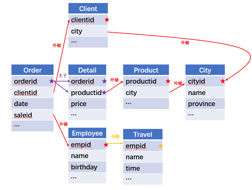
During data analysis, we may encounter mixed associations where homo-dimension, primary-sub, and foreign key associations occur at the same time, and it is when the associative relations are very complex and need to be clearly sorted out. For example:

 

Based on the order table, order detail table, product information table, employee information table, travel information table, client information table, and city information table, the task is to calculate the sale amount of Heilongjiang products sold in each province by post-90s salesman who travel for more than 10 days.

 

The associative relations are shown below:

 

Python

emp4 = pd.read_csv("D:\data\Employee4.csv") trv4 = pd.read_csv("D:\data\Travel4.csv") emp_inf = pd.merge(emp4,trv4,on=["empid","name"]) years = pd.to_datetime(emp_inf.birthday).dt.year emp_inf_c = emp_inf[(years>=1990) & (years<2000)&(emp_inf.time>=10)] clt4 = pd.read_csv("D:\data\Client4.csv") city4 = pd.read_csv("D:\data\City4.csv") sale_location = pd.merge(clt4,city4,left_on='city',right_on='cityid') pdt4 =   pd.read_csv("D:\data\Product4.csv") pdt_location = pd.merge(pdt4,city4,left_on='city',right_on='cityid') detail4 = pd.read_csv("D:\data\Detail4.csv") order4 = pd.read_csv("D:\data\Order4.csv") detail_pdt = pd.merge(detail4,pdt_location,on='productid',how="left") order_sale_location = pd.merge(order4,sale_location,on='clientid',how="left") order_sale_location_emp = pd.merge(order_sale_location,emp_inf_c,left_on='saleid',right_on='empid',how="left",suffixes=('_c', '_e')) order_inf = order_sale_location_emp[order_sale_location_emp.empid.notnull()] order_detail = pd.merge(order_inf,detail_pdt,on='orderid',how="left",suffixes=('_s', '_p')) order_detail_Hljp = order_detail[order_detail.province_p=="Heilongjiang"] res = order_detail_Hljp.groupby(['empid','name_e','province_s'],as_index=False).price.sum() print(res)

Employee table and travel table   Select the post-90s employees     Client table and city table   Product table and city table     Order detail and producing city Order and sale city   Order and employee     Order and order detail Select   Group and aggregate

 

There are many tables in this example with complex associative relations which are homo-dimension association (one-to-one), primary-sub association (one-to-many), and foreign key association (many-to-one), respectively. If there exists an association of many-to-many, it is most likely wrong, and the association needs to be rechecked, otherwise, many-to-many association probably leads to memory explosion. As for such complex associations, the best method provided in Python is to use the merge function to associate every two tables and parse each association step by step, which may be a bit troublesome but less prone to errors.

 

SPL

	A	B
…	…
43	=file("D:/data/Employee4.csv").import@tc()
44	=file("D:/data/Travel4.csv").import@tc()
45	=A44.join(empid,A43:empid,birthday)
46	=A45.select((y=year(birthday),y>=1990&&y<2000&&time>=10))
47	=file("D:/data/Client4.csv").import@tc()
48	=file("D:/data/City4.csv").import@tc()
49	=A47.join(city,A48:cityid,province)
50	=file("D:/data/Product4.csv").import@tc()
51	=A50.join(city,A48:cityid,province)
52	=file("D:/data/Detail4.csv").import@tc()
53	=file("D:/data/Order4.csv").import@tc()
54	=A52.join(productid, A51:productid,province:product_province)
55	=A54.group(orderid)
56	=A53.switch(orderid, A55:orderid;saleid, A46:empid;clientid, A49:clientid)
57	=A56.select(saleid).new(saleid.empid:empid,saleid.name:sale_name,clientid.province:sale_location,orderid.select(product_province=="Heilongjiang").sum(price):price)
58	=A57.groups(empid,sale_name,sale_location;sum(price):price).select(price)

 

SPL is quite capable to handle such complex associations, in which the homo-dimension, primary-sub, and foreign key associations are all very clear. SPL can also associate two associations simultaneously, which is very fast and less error-prone.

 

Summary

When performing foreign key association, Python still copies data, and only parses one association at a time. In addition, every association is independent, so the association created previously can not be reused later, instead, it has to be re-associated, which results in low efficiency in association.

 

On the contrary, SPL can reuse the associations that created previously, making the operation much more effective.