In data processing and analysis, SQL is basically in a position similar to “Standard English” and is almost a necessary ability to master. However, using SQL is inseparable from the relational database system, i.e., RDBMS. It’s like speaking standard English mainly occurs in English-speaking countries/regions. Of course, if you want to go to China, it's worthwhile to learn Chinese, for the reason that just as learning Python or Hadoop, as a skill, it will help you find a job. But, if you want to do analysis on general text data or Excel table, it’s like going to a small country like Kiribati, just for the convenience of shopping, is it necessary to learn local language by starting with practicing pronunciation, memorizing vocabularies and learning grammar? I’m afraid not, and the first thing that comes to your mind is probably to search online to find a useful translation tool.

On this issue, esProc can be said to be a must-have tool for staying at home and traveling!

In fact, although using SQL to process well-structured text or Excel table data is a lazy idea, it is a very natural train of thought. A file or table consists of several rows of data, and each row of data either uses a defined separator (space, comma, tab, etc.) to separate items or specifies the fixed length of each item. Such representation is almost the same as that of the table (Table) in a relational database, even the variable-length field and the fixed-length field seem to be similar. The difference is that the file does not have the concepts of primary key, data type, and null or non-null. In addition, the description of the relationship between files is not as clear as the database, and is often only used as the business rules or the experience, existing in the user's mind, or in some documents for you to reference.

esProc works in the same idea. By automatically parsing the structured text or Excel file, esProc maps the files to “table”, and on this basis, esProc fully supports the syntax and functions of SQL.

 

Well, without further ado, let’s get to the point. Take two associated files as an example to see how to easily perform the query and analysis without following the step "installing the database -> creating database table -> importing data":

First, let’s look at the data in this example, there are two files: employee information (employee.txt) and basic state information (state.xlsx). Note that we use two types of files here, one is the formatted TXT text, and the other is Excel spreadsheet, that is to say, esProc can connect different types of data sources at the same time, amazing? surprising?

What's more amazed is that esProc can automatically identify and read four types of files according to file suffix! They are: text (txt), Excel (xls, xlsx) and csv files.

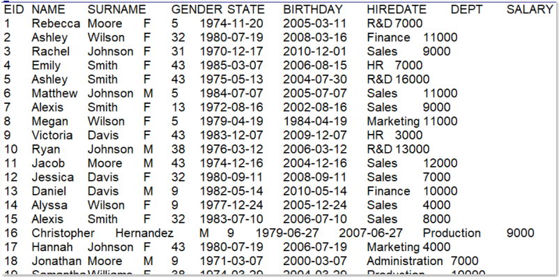
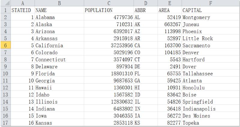
The following two figures are the data sample of employee information and state information respectively. The two files are associated by the STATE item (column 5) in employee information and the STATEID item (column 1) in state information.

Data sample of employee information:

Data sample of state information:

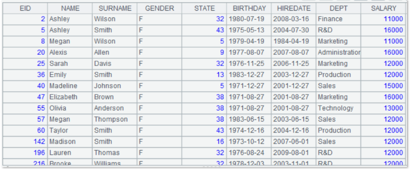
OK, let’s get started. First, perform the simplest single-table query to find out the female employees (GENDER='F') whose salary is greater than 10,000 (SALARY>10000), and the outputted results are sorted by employee ID (EID). The esProc code is as follows:

	A
1	=connect()
2	=A1.query(“select * from c:/sql/employee.txt where gender=’F’ and salary>10000 order by eid”)

Yes, you read that right - the code is simple and familiar like this! Step 1, connect to the database... well, no parameter is specified here, so the file system is connected directly; step 2, use the query() function to execute SQL query, and the SQL code here is exactly the same as that of database query except that the table name after from is replaced with the file name! The query results are as follows:

Note that in Windows System, the file path in esProc uses the slash "/" instead of backslash "\", which is consistent with Java language.

Well, it’s so similar, let's take a less similar example: query employees who were born no earlier than January 1, 1980 and whose salary is greater than 10,000:

	A
1	$()select * from c:/sql/employee.txt where BIRTHDAY>=date(‘1980-01-01’) and SALARY>10000

It's very simple. Using $() is equivalent to the connect() function, and you can code in SQL directly after it. In fact, different data source names can be written in the parenthesis so as to connect multiple data sources at the same time.

In addition, this example uses SQL’s date() function for converting the string to the date.

 

Then, it is the key to distinguish SQL database from a single file, that is, association query. When we want to find out the female employees whose salary is greater than 10,000 and which state she is in:

	A
1	=connect()
2	=A1.query(“select t1.eid eid,t1.name name,t1.gender gender,t2.name state,t2.population population,t1.salary salary from c:/sql/employee.txt t1 left join c:/sql/state.xlsx t2 on t1.state=t2.stateid where t1.gender=’F’ and t1.salary>10000 “)

Indeed, replacing the table name with file name is a bit long, therefore, we adopt the usage of alias in SQL, the result is shown as below:

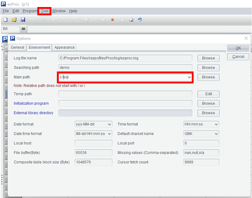
In addition to using the alias to replace the absolute path of file, it can configure the main path in esProc - Menu - Tools - Options if the path is particularly long or there are many files, so as to facilitate writing and clear reading. In this way, the file name or the relative path can be used directly in SQL, is it more like specifying a database and directly accessing the tables in it?

The configuration method is shown in the figure below:

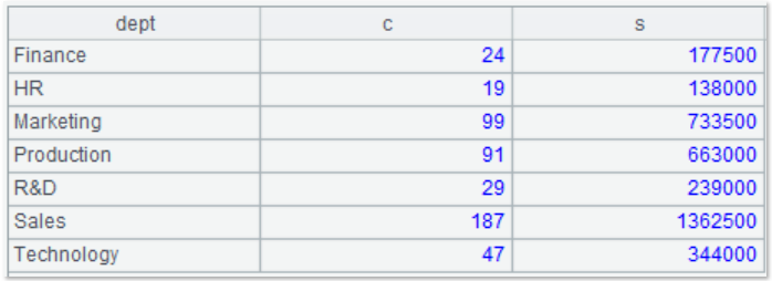
After configuring the main path, when we want to query the number of employees and the total salary of the departments with a total salary greater than 100,000, the query code is as follows:

	A
1	=connect()
2	=A1.query(“select dept,count(1) c,sum(salary) s from employee.txt group by dept having s>100000”)

Query results:

 

Next, let's look at some details:

1) esProc supports the logical operation and, or and not. For example, the following code is to query the male employees whose surname is Smith or Robinson and who are not in the Sales department:

	A
1	=connect()
2	=A1.query(“select * from employee.txt where (surname=’Smith’ or surname=’Robinson’) and gender=’M’ and not dept=’Sales’ “)

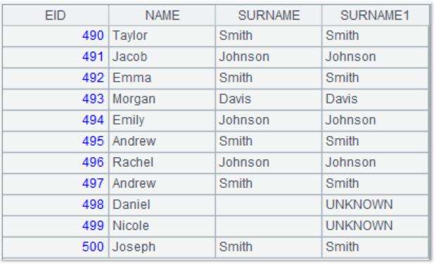
2) esProc supports the use of is null to judge whether it is null, and of is not null to judge whether it is non-null, for example: find out the employee whose surname is null:

	A
1	=connect()
2	=A1.query(“select EID,NAME,SURNAME from employee.txt where surname is null”)

Also, esProc supports the use of the coalesce function to process null value. For instance, when the surname field of employee is null, it is displayed as “UNKNOWN” in the result:

	A
1	=connect()
2	=A1.query(“select EID,NAME,SURNAME,coalesce(SURNAME,’UNKNOWN’) as SURNAME1 from employee.txt”)

Query results are as follows:

Note: The field alias in the esProc cannot be the same as the field name in the file.

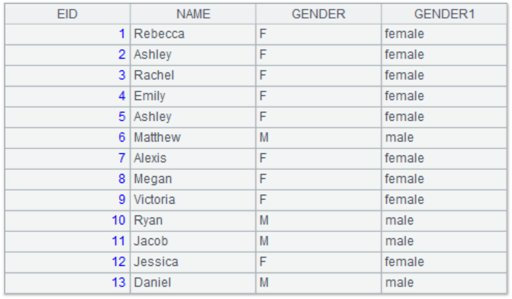
3) esProc supports Case when, for example, if the gender field is “F”, it is to be displayed as "female", and in the case of “M”, it is to be displayed as "male".

	A
1	=connect()
2	=A1.query(“select EID,NAME,GENDER,(case gender when ‘F’ then ‘female’ else ‘male’ end) as GENDER1 from employee.txt”)

The query results are as follows:

4) esProc supports the like keyword for fuzzy query, for example: to query the employees whose surname field contains "son".

	A
1	=connect()
2	=A1.query(“select * from employee.txt where surname like ‘%son%’”)

where, “%” is the wildcard, representing one or more characters. In addition, “_” represents a character. If you want to query the employees whose surname ends with "son" and there are three characters before "son", you can write: surname like ‘___son’; "[WJ]"represents the character list containing"W"and"J"; surname like '[WJ]%' represents that the surname starts with "W"or"J"; surname like '[!WJ]%' represents that the surname does not start with "W"or"J".

5) esProc supports the use of In keyword to query the data in multiple values. For example: query the employees of the three departments "Finance, Sales, R&D".

	A
1	=connect()
2	=A1.query(“select * from employee.txt where dept in (‘Finance’,’Sales’,’R&D’) “)

6) esProc supports defining an external table through with T as (x). For example: the name and population of each employee's state can be found by left-joining the state field in the employee.txt with the stateid field in the state table of another data source, i.e., demo database:

	A
1	=connect()
2	=A1.query(“with t2 as  (connect(\”demo\”).query(\”select * from states\”)) select t1.eid eid,t1.name name,t1.gender gender,t2.name state,t2.population population,t1.salary salary  from employee.txt t1 left join t2 on t1.STATE=t2.STATEID”)

In this SQL code:

with t2 as  (connect(\”demo\”).query(\”select * from states\”)) defines an external table t2 to connect the demo data source (it is actually the hsql demo database that comes with esProc), and uses the query function to execute the SQL "select * from states" (where, \” is the escape writing method of using double quotation marks in a string).

The following “select t1.eid … left join t2 on t1.STATE=t2.STATEID” uses the defined t2 to left join the employee.txt to find out the name and population of each employee's state.

This query is the typical joint query of a database and a text file. In fact, the with keyword can define the data queried from various data sources, hereby achieving the joint query across different types of data sources very flexibly.

7) esProc supports outputting the query results to the file through into. For example: query the number of employees and the total salary of the department with a total salary greater than 100,000, and write the results to deptResult.xlsx. Here, the new file is like a new table in the relational database.

	A
1	=connect()
2	=A1.query(“select dept,count(1) c,sum(salary) s into deptResult.xlsx from employee.txt group by dept having s>100000”)

Having introduced so many functions of esProc, it can be concluded that through esProc, it can basically achieve the easy and direct use of SQL on structured text data (txt, csv, etc.) and Excel files (xls, xlsx).

Of course, esProc doesn't replicate SQL's capabilities “as is”. For example, esProc cannot directly support the subqueries in SQL at present, but will solve it in a more flexible, convenient and intuitive stepwise calculation fashion. Moreover, for some special join calculations, esProc is a bit slower than conventional databases.

 

Finally, let's take a look at some additional benefits that can be obtained by SQL calculations through esProc:

1) Dynamic calculation based on input parameters:

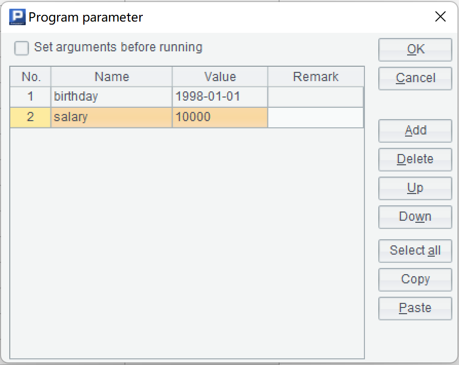
When querying the data, it often needs to calculate based on different conditions, which is what we call dynamic execution. At this point, we can define "cellset parameters" to reserve places for conditions that may change. For example, when we want to find out the young employees with higher salary in the company, but the age range and salary starting point are still uncertain, in this case, we can define two parameters: birthday and salary in esProc IDE’s menu "Program / Cellset Parameter":

And then code in SQL with the placeholder "?" in the query statement, and specify in order the corresponding cellset parameter name as input:

	A
1	=connect()
2	=A1.query(“select * from employee.txt where BIRTHDAY>=? and SALARY>?”,birthday,salary)

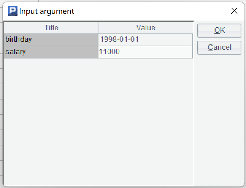
If the specific value is specified when defining the cellset parameters, and the "Set arguments before running" is not checked, then the specified value will be used directly while running the script. If "Set arguments before running" is checked, the "set argument value" window will pop up every time the script is run. In this way, we can enter the argument value we need at any time, and the query results will change accordingly:

2) Querying files using SQL in the command line

In Windows or Linux system, we can also query the file data directly by calling the written esProc script in the command line. If the schedule mechanism of the operating system is used, the data calculation in batches can be performed at the specified time.

We first look at an example that does not return a result set. When we want to provide the finance department with number of employees and total salary of department having a total salary greater than 100,000 on a regular basis, and store the results into deptResult.xlsx (which can then be sent to relevant personnel by mail or other means), follow the steps below:

First, code the esProc script and save it as deptResult.dfx.

	A
1	=connect()
2	=A1.query(“select dept,count(1) c,sum(salary) s into deptResult.xlsx from employee.txt group by dept having s>100000”)
3	>output(“create deptResult.xlsx successfully!”)

Then, execute the esprocx.exe command (under the bin folder of esProc installation directory) in the command line, the execution result:

| C:\Program Files\raqsoft\esProc\bin>esprocx.exe deptResult.dfx

create deptResult.xlsx successfully! |

where, the second line is the prompt information outputted by output function, which can be used for monitoring the program execution and debugging.

 

Let's look at an example that returns a result set. The query requirements are the same, but it is not required to output the results to a file, instead viewing the results directly. This time, we change the name of the written esProc script and save it as deptQuery.dfx.

	A
1	=connect()
2	=A1.query(“select dept,count(1) c,sum(salary) s from employee.txt group by dept having s>100000”)
3	return A2

Execute and view the results in command line:

Furthermore, esProc can also code complete SQL statement directly in command line, and return the query results directly in the form of file. Is that as convenient as a database command line query tool?

First define a parameter sql to transfer the SQL statement to be queried.

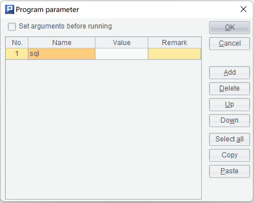
Then code the following esProc script and save it as query.dfx,

	A
1	=connect()
2	=A1.query(sql)
3	return A2

When executing the command, code the SQL statement directly in the command line, and the result is as follows:

Combing the aforesaid approach of dynamic calculation based on parameters with the calculation in command line, a certain degree of interaction can also be achieved. Again, we use the example of finding out the young employees with higher salary:

Define two parameters: birthday and salary in esProc IDE menu "Program / Cellset Parameters":

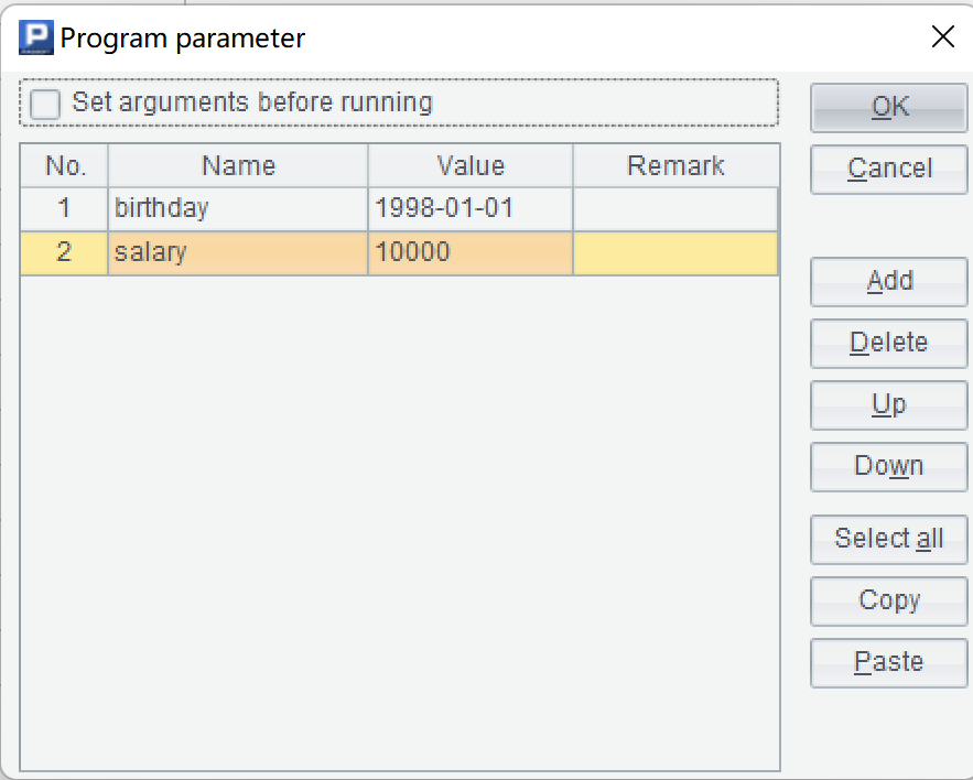
Code the following esProc script and save it as empQueryParam.dfx,

	A
1	=connect()
2	=A1.query(“select * from employee.txt where BIRTHDAY>=? and SALARY>?”,birthday,salary)
3	return A2

When executing the command, provide the values for the two parameters in order, and the results are as follows:

 

Up to this point, we have fully understood that, with the esProc, we can use SQL, a suitable tool, to process the data files. In fact, the esProc is the real suitable tool in this regard! In addition to the way of processing the data files directly as "tables" described in this article, the truly powerful functions of esProc are far more than that. With this lightweight data analysis tool, the data whether in database or in file system can be easily processed, hereby solving the data processing problem in an effective and quick way!