

External storage index of SPL
Established outside the original table, the external storage index is an association table between the value of to-be-searched (TBS) field and the physical position of original table record. When searching, we can use a specified value to quickly find the physical position of original table from the association table, and then read the original table record.
Thus, the index will store many TBS field values. To find the specified value in these values, the search action originally used for the original table will also be utilized. Therefore, we need to design a special index structure to improve the search speed inside the index.
Hash index
The hash index of external storage refers to calculating the hash value of TBS field of original table first, and then storing the values of TBS field and their corresponding physical position in original table in turn by the hash value. In this way, records with the same hash value will be stored together.
Usually, the data amount of original table is very large, and the index is also too large to be stored into memory. To address this situation, we need to create a small index for the index itself. Take the data table of external storage as an example; the process of creating hash index for the primary key id field is shown as below:
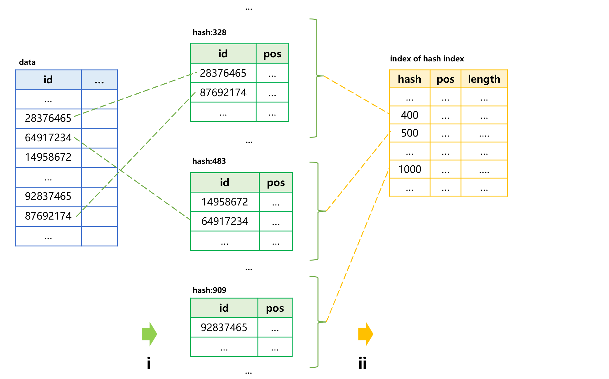
Figure 1: Creating hash index
Step i, calculate the hash values of id field of the data table first, and then store them into the hash index of external storage in segments according to their order. Since we know the hash value range in advance, the number of segments to be divided can be determined. For example, the hash values 1-100 are stored into one segment and the hash values 101-200 are stored into another segment to ensure each segment is small enough so that it can be loaded into memory. step ii, save a small index with a fixed length at the header of the hash index to record the range of hash values stored in each segment, as well as the physical position and length of each segment.
Once the hash index is created, we can search for the specified id through the index. The general process is as follows:
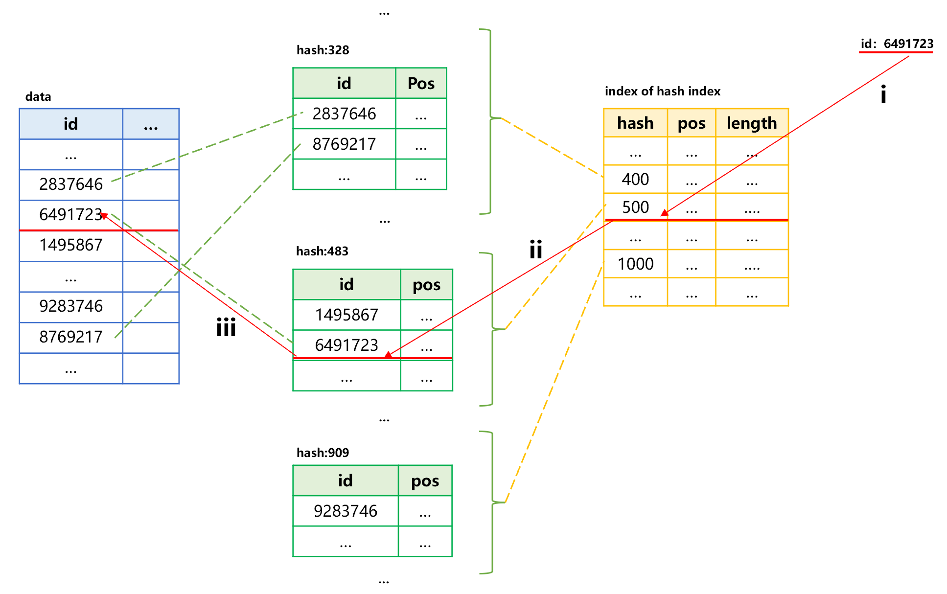
Figure 2: Search using hash index
Step i, calculate the hash value based on the specified id value 6491723; the calculated hash value is 483, which is in the segment of 401-500; read the small index into memory to search for the starting position and length of this segment. In this case, we can utilize the in-memory search technology. Since the hash values of each segment are stored in order, the binary search can be used. If the number of hash values of each segment is fixed, we can also use the sequence number to position record.
Step ii, read this segment of hash index into memory, and use the in-memory search technology to find the record whose id value is 6491723 so as to obtain its corresponding position in original table.
Step iii, utilize the position to read the target record in original table.
In this way, the target value can be found by reading three times in an order of small index, hash index segment and original table. Moreover, the small index can reside permanently in memory, eliminating the need to read it repeatedly when searching multiple times.
The above situation is based on the premise that the small index can be loaded into memory. When the amount of data is large, however, the small index may be so large that the memory cannot hold. In this case, we need to create smaller index for the small index, which means that the index may be divided into multiple levels. We represent the number of index levels with the loading order. Specifically, the initially loaded minimum index section is called the first-level index, which is used to find the appropriate second-level index,, and then the third- and fourth-level indexes. Generally, four index levels are already large enough, enabling us to locate the physical position of target value at the last level. The maximum number of reads per search is the total number of index levels, plus one that reads target value. The first-level index can also reside permanently in memory without the need to read repeatedly.
The problem of hash index is that we may have bad luck and encounter a situation where the hash function does not evenly distribute the records, resulting in a failure to store records into one index segment due to too many records in a certain slice of hash values. For example, there are too many records with hash values between 401 to 500 in figure 1, making one index segment unable to hold. In this case, we need to do the second round of hashing, and use another hash function to redistribute the records. If we encounter an unfavorable situation again, we may need to do the third round of hashing, the fourth round……, as a result, the number of hash index levels is not fixed, and there may be more levels for some search values.
The SPL code for creating and using hash index to search is roughly as follows:
| A | |
|---|---|
| 1 | =file("orders.ctx").open() |
| 2 | =file("orders.idx") |
| 3 | =A1.index(A2:1000000;id) |
| 4 | =A1.icursor(;id==123456;A2).fetch() |
A3: create an index for composite table of A1; the TBS field is id; the index file is orders.idx. When creating a hash index, it needs to give a hash value range (1000000 in this code).
In A4, we can use corresponding index file to search in A2.
The sorting index
Sorting index is more common in external storage.
Hash index can only do the equivalence search for the search value, that is, the judgment condition is “be equal”; it cannot do the interval search, which means the judgment condition is that the TBS key is in a specified interval. Moreover, when using hash index to search, the second round of hashing may be required if an inappropriate hash function is encountered, resulting in unstable performance. Sorting index can solve these problems.
The principle of the sorting index is to store the values of TBS key in order in the index, and then use binary search to find the physical position of target value corresponding to the search value. For this scheme, both equivalence search and interval search can be performed.
In practice, we cannot simply perform a binary search on the index directly. Instead, similar to hash index, we need to divide the sorting index into several segments and establish a small index for these segments. When searching, first read the small index, and then use binary search to find the index segment corresponding to the search value, and finally read the index segment to find the physical position of target value. Likewise, the small index can reside permanently in memory to reduce the amount of reading.
As with the hash index, the sorting index needs to be divided into levels when the amount of data is huge. However, since the sorting index can determine the number of records stored in each index segment in advance, the second round of hashing caused by bad luck in hash index will not occur. If each level stores 1K records, then four levels can store 1K*1K*1K*1K=1T records, which is more than enough. Generally, three levels are enough.
When using a sorting index to do an equivalence search, the binary search needs to be performed in every index level, which is slightly slower than the direct positioning way of hash index. However, since most of the time to search external storage is spent on the data reading rather than the CPU operation, there is little difference between the two kinds of indexes. Due to the wider adaptability of the sorting index, the majority of external storage indexes are the sorting index. Hash index is only used in very few scenarios that require extreme performance and that only need equivalence search. Unless otherwise stated, the external storage index mentioned below are all the sorting index.
The default index of SPL is the sorting index.
| A | |
|---|---|
| 1 | =file("data.ctx").open() |
| 2 | =file("data.idx") |
| 3 | =A1.index(A2;id) |
| 4 | =A1.icursor(;id==123456;A2).fetch() |
| 5 | =A1.icursor(;id>=123456 && id<=654321;A2) |
If no hash range is specified in the index() function, then an sorting index will be created.
In A5, we can also perform an interval search based on the sorting index.
The reason why we create a sorting index instead of sorting the original data table directly by the TBS field is mainly because that the index occupies less space. The index has only the TBS field and physical position and is equivalent to a data table containing two fields, while the original data table often contains dozens of or even more than one hundred fields and is much larger than the index; if the whole table is sorted, it will take up at least twice the space.
Moreover, even if the data is ordered, searching the original data table with binary search algorithm still cannot obtain better performance than index. As mentioned earlier, direct binary search has no multi-level index, and nor can it locate precisely and, it involves many futile reading actions. Simple binary search is usually used in scenarios where performance requirements are not very high and we do not want to maintain an index. Although the index is smaller than raw data, it still occupies considerable space and needs to be updated at the same time when appending data.
The creation of index is essentially a sorting action. The creation of hash index is also a sorting action in essence, except it is sorted by the hash value of TBS field.
Sometimes we need to use two fields as the TBS key, which does not differ from a single field theoretically, except that comparison action is a little complicated. However, having understood the essence of index, i.e., the sorting, it helps the creation of such index.
For example, when we want to search both the city and birthday fields in the user table, we can create an index for the two fields respectively, as shown in the figure below:
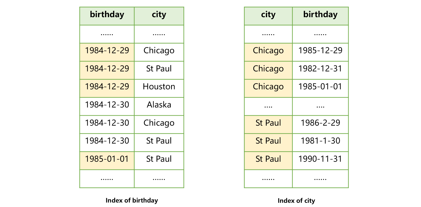
Figure 3: Creating an index for two fields respectively
Doing so is helpful for searching by two conditions, i.e., birthday and city, but only one index can be used. For example, after using the index of birthday in figure 3 to find the users born on 1984-12-29, we found that these records in the city field are not ordered, therefore, we cannot use this index to search for St Paul.
Alternatively, we can create a joint index on the two fields, as shown in the figure below:
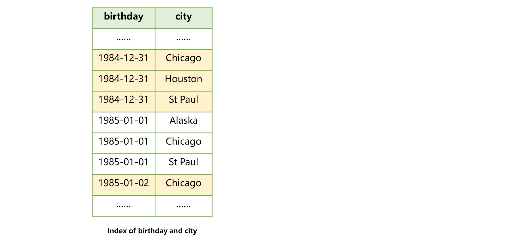
Figure 4: Joint index of birthday and city
This joint index allows us to search the birthday field first and then the city filed or, we can search the birthday field only. However, we can’t use the index to search the city field only, nor can we search the city field first and then the birthday field.
If space permits, we can build two joint indexes as below. In this way, we can utilize the index to search any one field or any two fields:
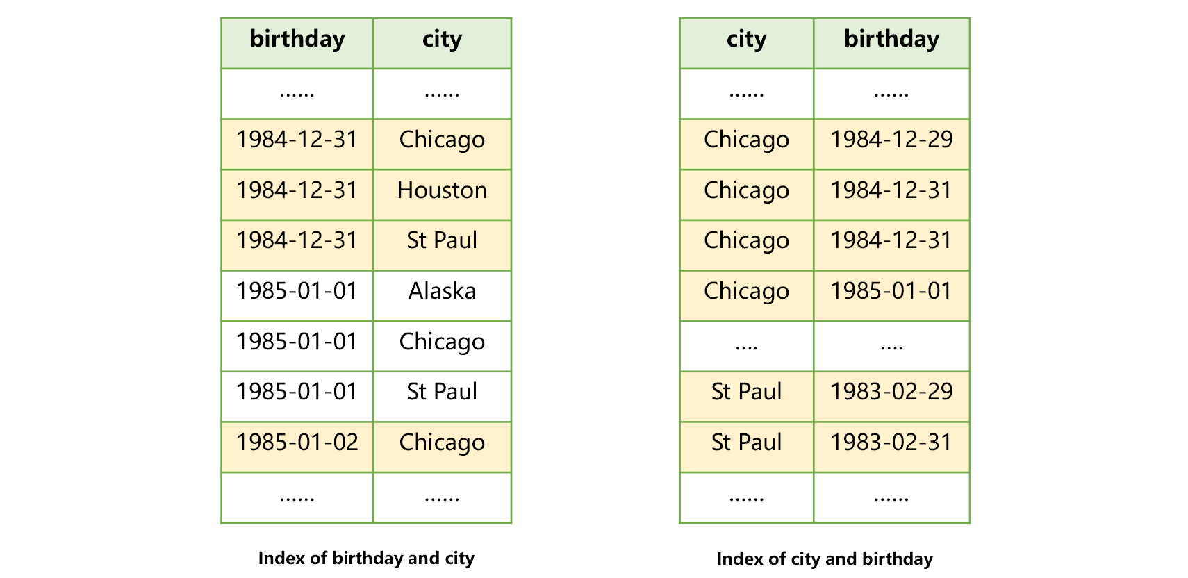
Figure 5: Recommended joint index
When multiple indexes are available for use, SPL provides the mechanism of automatically finding the most appropriate one. We can refer to the above methods to find the most appropriate index from existing indexes to improve the search speed.
Loading in levels
The index of big data is usually very large, so there is a need to establish multi-level index. Each time we perform a search task, only by reading the index level by level can we finally locate the target value.
Some indexes need to be used hundreds of times repeatedly. If such indexes are reloaded every time they are used, you will feel an obvious delay.
SPL provides a mechanism of automatically caching the indexes, which will cache the index that is already used. When the cached index is used again in a short time, it will not be read, hereby effectively reducing the search delay. Moreover, SPL also provides a method of actively preloading some index segments, that is, it will load part of index segments actively when the system starts. As a result, the subsequent search will be faster without having to wait until all index segments are accessed.
The index levels of SPL composite table have a maximum of four. Take three-level index as an example, if the memory space permits, then the more the number of preloaded levels, the better the performance. The following figure shows the general process of loading the composite table index in levels:
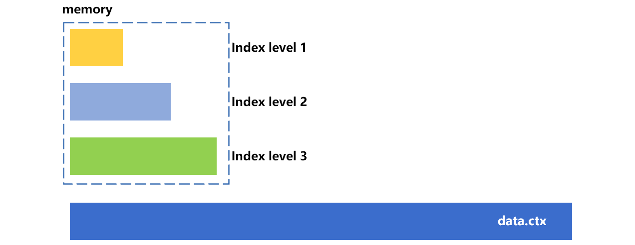
Figure 6: Loading in levels
Each index level is equivalent to 1K TBS values; four levels can support up to 1T records. The first three index levels may occupy about several gigabytes of space. After loading the first three index levels, there is no need to read the index segments again for composite tables with records number of no more than 1G, and it only needs to read them one more time for composite tables with larger data amount.
The SPL code to actively preload index levels is roughly as follows:
| A | |
|---|---|
| 1 | =file("data.ctx").open() |
| 2 | =file("data.idx") |
| 3 | =A1.index@3(A2) |
| 4 | =A1.icursor(…;id==123456).fetch() |
@3 means the index segments at the first three levels are preloaded into memory and reside permanently in memory.
If there is no enough memory space, we can use @2 to load only two levels.
The preloaded index segments will exist throughout the search process and will be automatically used by other threads of the same process.
Batch search
When using the index to search the external storage, in addition to single search value discussed above, there is another situation where there are multiple search values, i.e., batch search. If the multiple search values are searched in memory, searching multiple times will be OK. When searching multiple values in external storage, because the time to read hard disk is much longer than that of processing judgment, it is often worthwhile if the subsequent searches can reuse the results read in previous search, even if the judgment time increases due to the complex code. Therefore, a more detailed optimization scheme is meaningful for multiple search values.
Let’s take a look at the process that uses the sorting index of external storage to implement batch search. Assuming that the id field of the data table is natural number; the sorting index of data has two levels; the first level can be loaded into memory; the first index segment of the second level corresponds to the id range 1-100, the second segment corresponds to 101-200, and subsequent index segments follow the same id range rules.
Now we want to use the index to search for n given values transferred by the frontend through parameter. For ease of understanding, we assume four values, 143, 98, 177 and 355 are transferred. The search process for the first value 143 is roughly as shown as below:
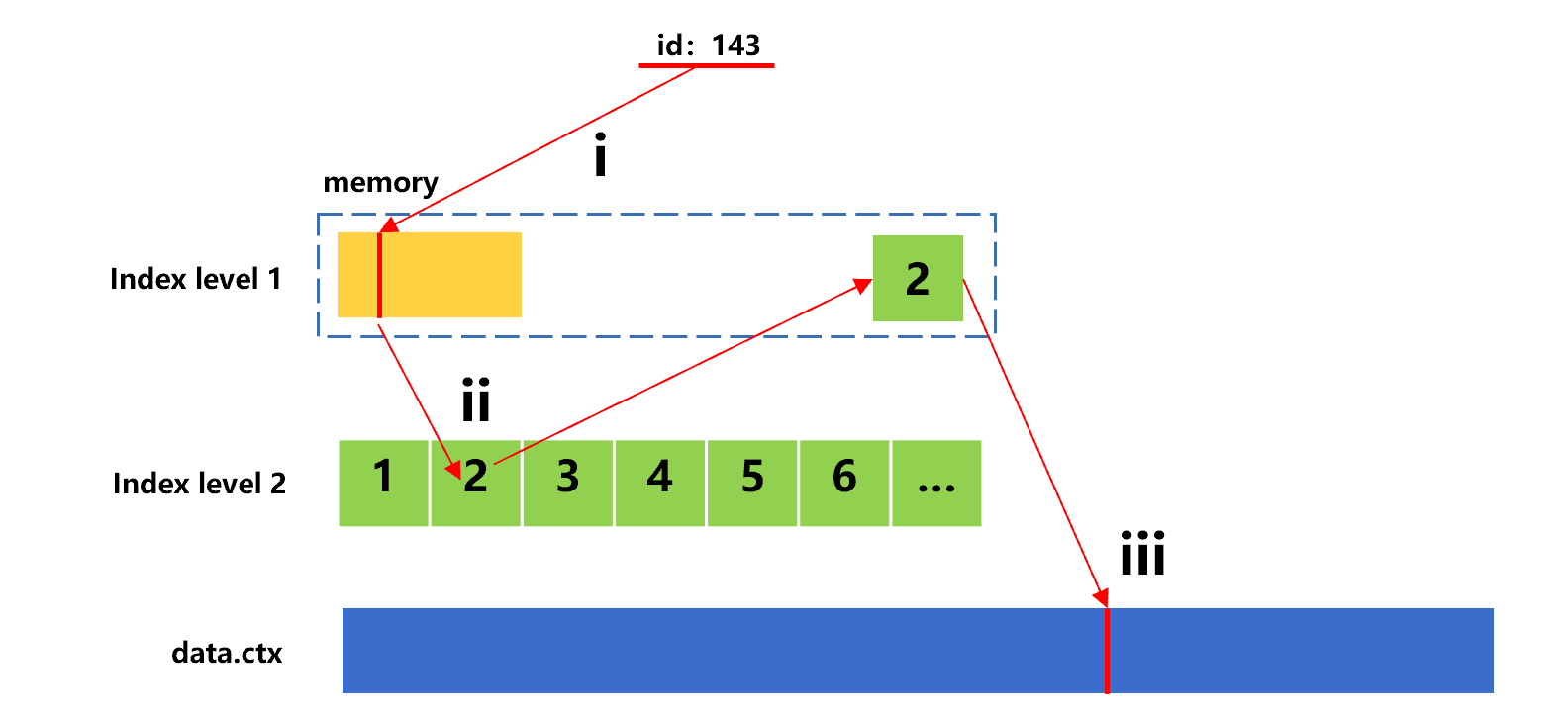
Figure 7: Search for the first value with sorting index
In this search, since the id value 143 is in the second index segment of index level 2, step ii needs to read this segment from hard disk.
The following figure shows the search process for the second value 98.
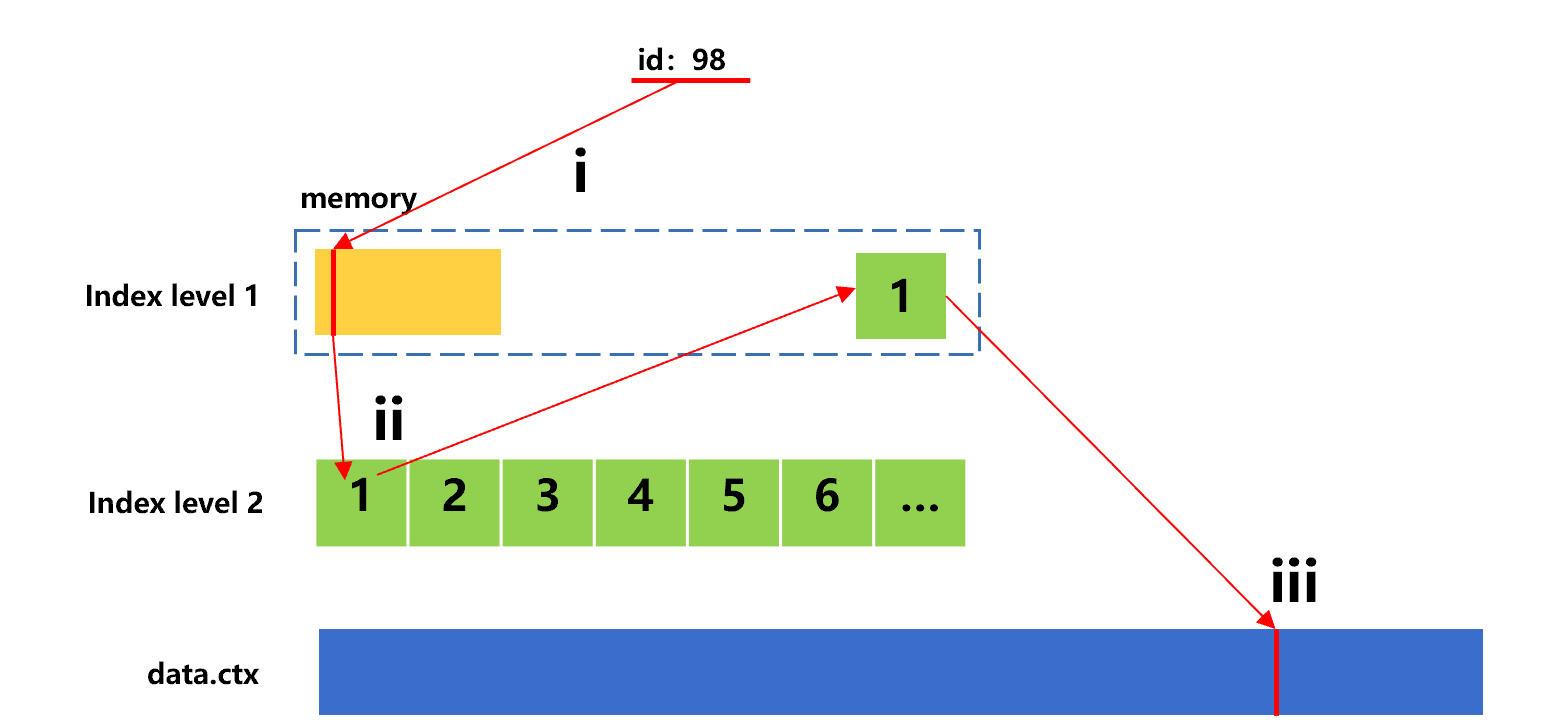
Figure 8: Search for the second value with sorting index
The id value 98 is in the first index segment of index level 2, and hence step ii needs to read this segment from hard disk.
The following figure shows the search process for the third value 177.
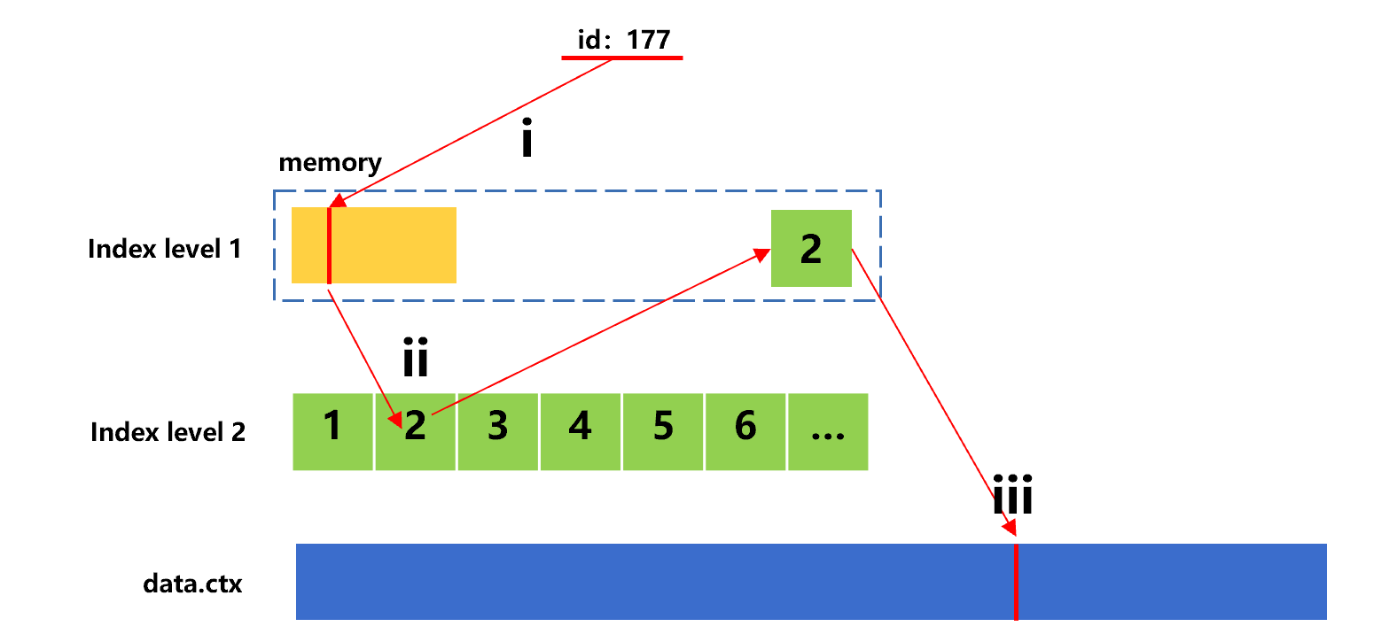
Figure 9: Search for the third value with sorting index
As can be seen that the id value 177 is also in the second index segment of index level 2, and step ii needs to read this segment once again from hard disk. Therefore, a phenomenon of repeatedly reading the same index segment occurs.
In practice, the number (n) of given values may be very large, and hence this phenomenon will occur very frequently.
To reduce the number of reads, we can cache both the 2nd and 1st index segments used for searching for 143 and 98 respectively. In this way, we can reuse these cached data to reduce the number of reads when searching for 177. However, when n is very large, we will find that many index segments may need to be cached. Since we can’t predict which cached index segments will be used in the future, we have to discard some of them sometimes as too much cached data will occupy a lot of memory space. As a result, the said phenomenon may occur in subsequent searches.
SPL provides an optimization scheme for batch search. When we sort multiple given values and then search them in sequence, we can avoid the said phenomenon in principle. For example, the sorted four given values are in the order of 98, 143, 177, 355. The search process for the first value 98 is roughly as shown below:
Figure 10: Search for the first value with sorting index after optimization
The process to search for the second value 143 is shown as below:
Figure 11: Search for the second value with sorting index after optimization
The process to search for the third value 177:
Figure 12: Search for the third value with sorting index after optimization
In this figure, the id value 177 is also in the second index segment, we can continue to use the second index segment that has been read during searching for 143, avoiding repeated reading.
Since the given values are ordered, the latter value 177 is surely greater than the previous value 143. Moreover, the indexes are also ordered by the search field, and hence the index segment used to search for 177 will definitely not appear before the index segment of 143. If the index segment being used happens to be the one read in last search, this index segment can be used directly. If not, it can be determined that subsequent searches will never use the index segment read earlier, which completely avoids repeated reading.
SPL index has up to four levels. Once the optimization scheme is adopted, the cached index segments will not be too large as long as the required index segments are loaded step by step from the first level, making it easy for memory to hold. In this way, it can ensure that repeated reading caused by the discarding of cached data will never occur. The more the batch search values, the greater the overall advantage.
In fact, in figures 10, 11 and 12, after the position of 98, 143 or 177 in index segment is found in step ii, we cannot perform step iii immediately (read data from original data table). Instead, we need to find the positions of all 4 target records, and then sort the 4 positions before performing step iii.
The reason is similar. The original data table is usually stored in blocks and one data block is read at a time; if two target values are in the same block, they only need to be read once. After sorting by position, it is easy to reuse the data block of target value. Otherwise, the repeated reading of data block in the original data table may also occur, resulting in a waste of time.
These algorithms are already built in SPL. SPL code:
| A | |
|---|---|
| 1 | =file("data.ctx").open() |
| 2 | =file("data.idx") |
| 3 | =10000.id(rand(1000*10000)+1) |
| 4 | =A1.icursor(…;A3.contain(id);A2).fetch() |
A3: randomly generate a large number of id values.
A4: use contain as the batch search condition, and icursor function will sort the values in A3 first and then execute the optimization method described earlier.
In addition, even if the preloaded index of SPL is used, it still makes sense to sort the search values when the four-level index segments are required due to the large amount of data. At this time, the first three levels are preloaded and will not be read repeatedly. Since there are too many index segments in the index level 4, they can only be read instantly. Moreover, since the first three levels already occupy a lot of memory space, the index segments in the index level 4 will be discarded after they are used to reduce the memory occupation. As a result, repeated reading may still occur when the search values are out of order, and will account for a more obvious proportion in the entire search process after the first three levels are cached.
Columnar storage index
Columnar storage is a common means to improve performance. When the index technology is adopted, the columnar storage differs greatly from the row-based storage. For the data stored in row-based storage format, the position recorded can be represented by one number, yet for the columnar storage, each column has its own position; if all columns are stored in the index, too much space is required, even exceeding the original data.
SPL index for columnar storage does not record the position of each column, only records the internal sequence number, through which all columns can be found quickly. For example, the user table contains fields such as id, name, gender. The process of creating an index for the id field of user table in columnar storage format is roughly shown as below:
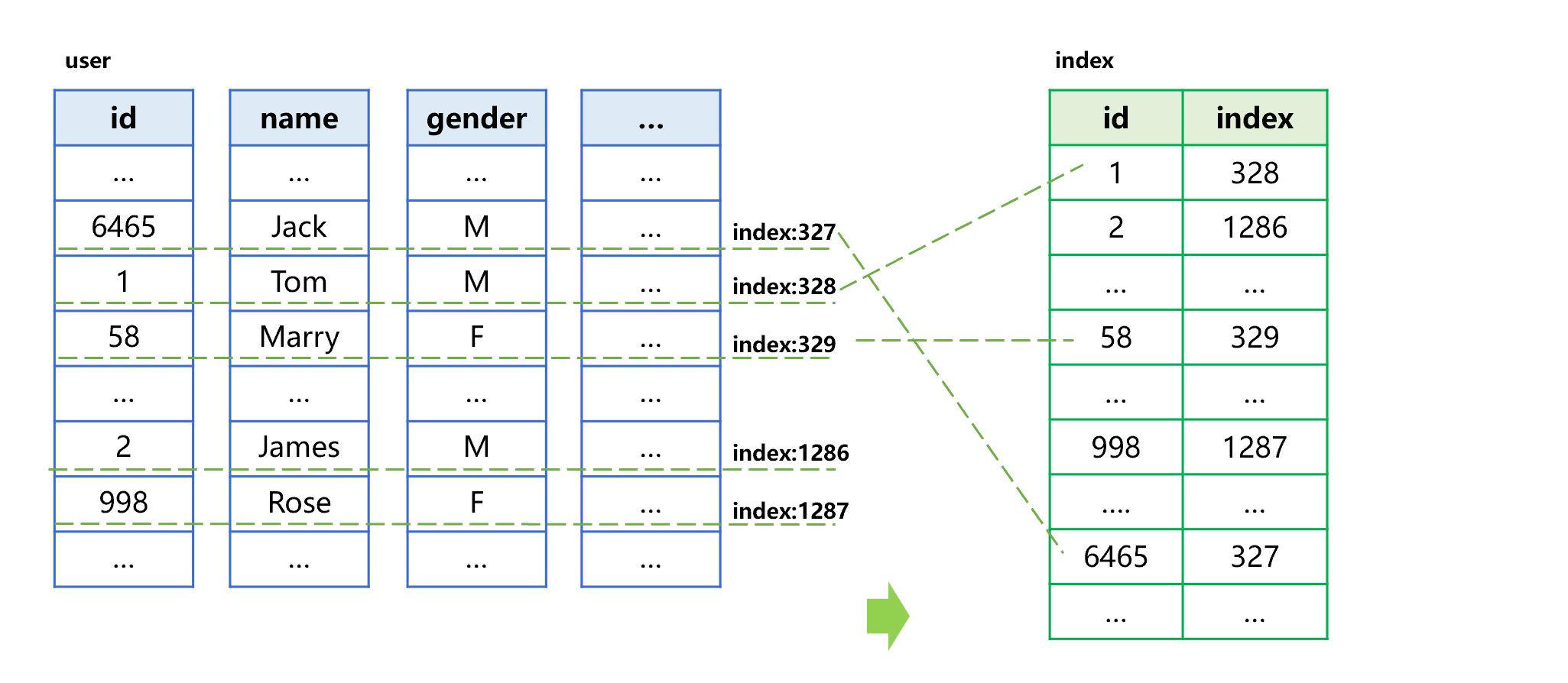
Figure 13 Generating columnar storage index
The process of generating a columnar storage index is divided into two steps: i)sort by the id field; ii) store the sorted values together with their corresponding sequence number in the original table into the index. For example, the first id value in the index is the minimum value 1, and its corresponding record is at the 328th row in the user table, then store the sequence number 328 into the index. In the same way, store other id values and sequence numbers in sequence to generate a final index.
The following figure roughly describes the process of searching by index:
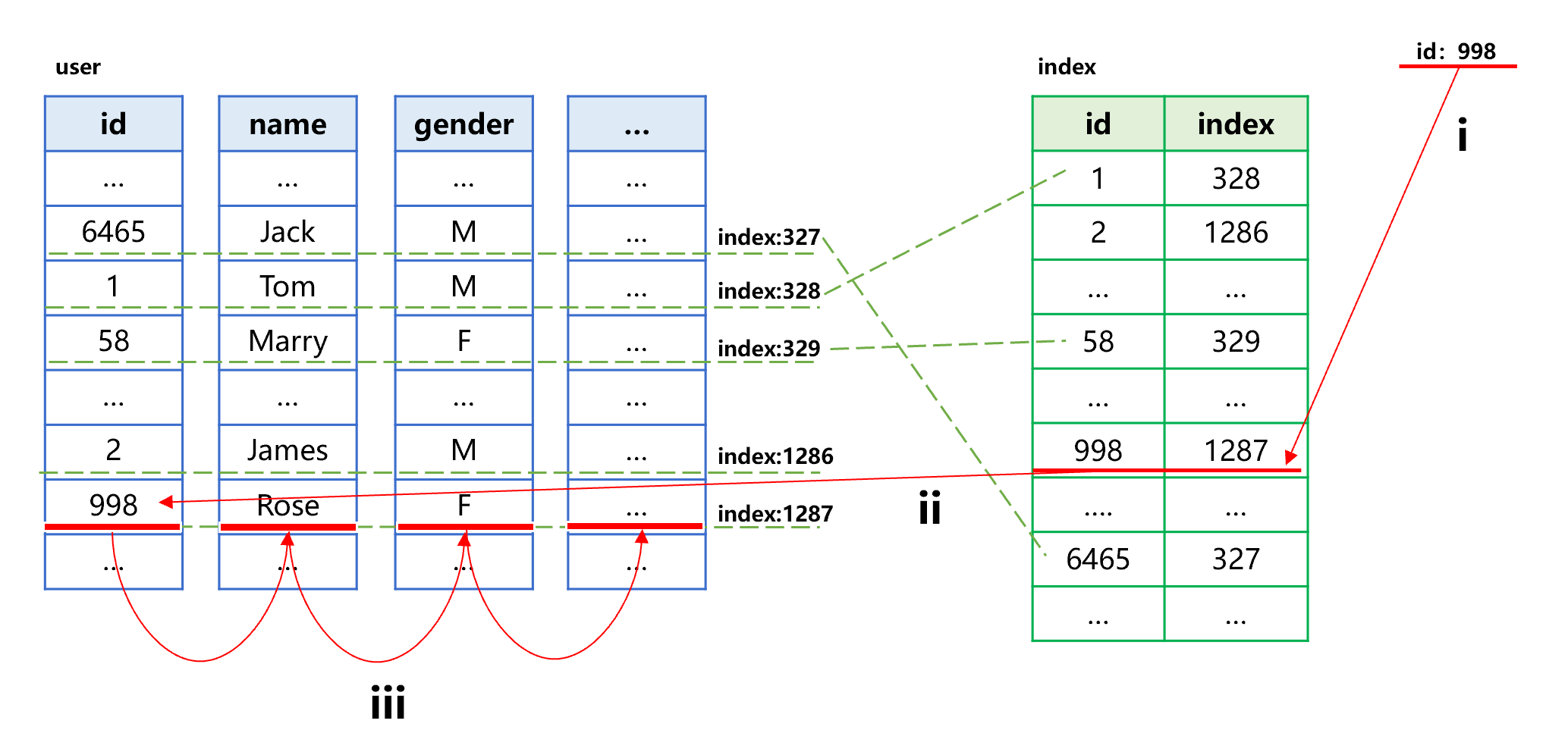
Figure 14: Search by columnar storage index
To search the specified id value 998, follow the steps: i)find id value 998 in the index to obtain the sequence number of its corresponding record in original table, which is 1287; ii) and iii), read the corresponding field value in the data area of each column of original table based on the sequence number 1287.
The columnar storage of SPL adopts the double increment segmentation technology, which can quickly find each field value based on the sequence number. However, the columnar storage is still much slower than row-based storage that reads directly by position. We can see from figure 14 that when reading the original table, it needs to read the data area of every column. Since the reading of hard disk requires a minimum reading unit, it will cause a situation that the amount of reading all columns will far exceed that of reading row-based storage. Moreover, the data in column storage format is usually compressed, the number of times we need to decompress is as many as the number of columns to read. Overall, the search performance of columnar storage is not as good as that of row-based storage.
Columnar storage is suitable for traversal calculation, while the row-based storage is more suitable for searching for the given value.
Index with values
SPL provides the “index with values” technology, allowing us to copy the values of other fields when creating the index. For example, the process of generating an index-with-value for the columnar storage user table is roughly shown as below:
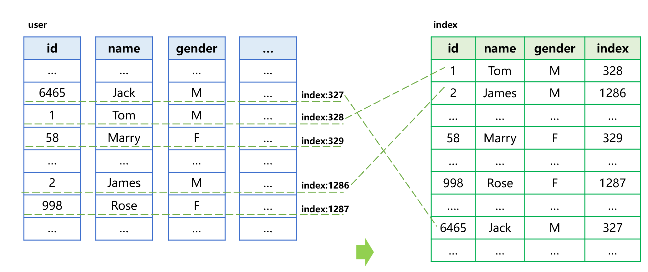
Figure 15 Generating an index-with-value
Different from ordinary index, the index-with-value provides the name and gender fields required by query, in addition to the sorted id and original table sequence number.
The following figure describes the search process by index-with-value:
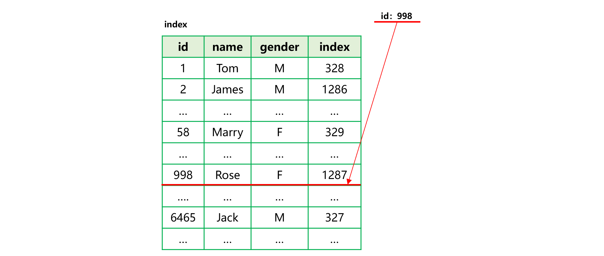
Figure 16: Search by index-with-value
This index adopts the row-based storage and stores the name and gender fields. If only the two fields are used when searching, there is no need to access the original composite table, which is equivalent to searching the row-based storage data, and hence a better performance can be obtained.
In this way, the original composite table can continue to adopt the columnar storage for traversal, while the index-with-value is used for searching and calculating the given value. As a result, the overall performance is improved, and the application scope is expanded. The disadvantage of index-with-value is that it will take up more storage space since more field values are stored.
The code of index-with-value is roughly as follows:
| A | |
|---|---|
| 1 | =file("user.ctx").open() |
| 2 | =file("user.idx") |
| 3 | =A1.index(A2;id;name,gender) |
| 4 | =A1.icursor(id,name,gender;id==998;A2).fetch() |
| 5 | =A1.icursor(id,name,gender;id>=123456 && id<=654321;A2) |
A3: when creating an index in A2, writing the fields to be referenced into the parameter of index function enables the field values to be copied in the index.
A4 and A5: when fetching the target values, there is no need to read the original composite table as long as the involved fields exist.
Sort by index
As mentioned earlier, the creation of index is essentially a sorting action. SPL provides a technology that utilizes existing index to sort the data table by the corresponding field. For example, there is already an index ordered by id for the data table; the process that utilizes this index to sort the data table by id is roughly shown as below:
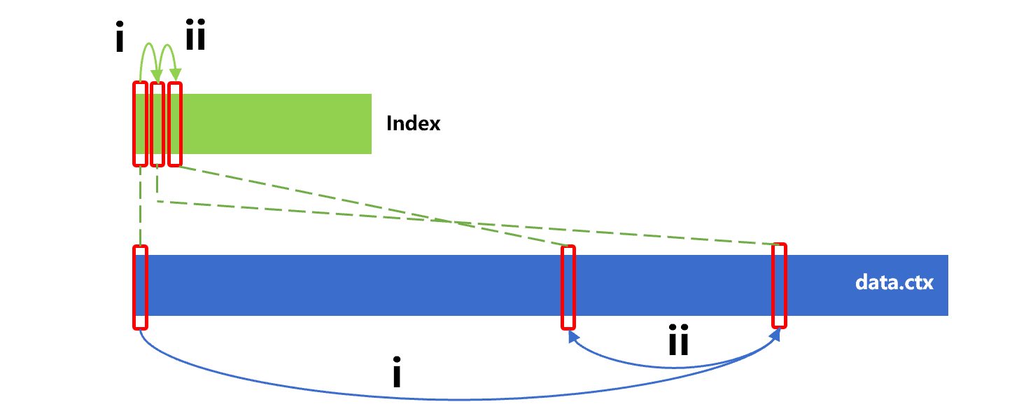
Figure 17 Sort by index
The process is divided into two steps, i)read the index in sequence; ii) read the original records in the original table according to the physical position of records stored in the index. Since the index is ordered by id, the read result is also ordered by id.
It can be seen from figure 17 that read on the index is continuous. However, since the original table is not ordered by id, the read on original table at step i and step ii is discontinuous. Moreover, since the reading of hard disk requires a minimum unit, a lot of irrelevant content will be loaded when reading discontinuous data, resulting in a significant performance decrease. Overall, this technology is likely to fail to obtain a better performance compared to performing big sorting directly on the original table.
However, sorting by index has its own advantage in that it can quickly output data. In contrast, the big sorting algorithm needs to traverse all data and generate the buffer files of external storage before outputting the data, resulting in a longer waiting time.
In some scenarios, this advantage can come into play. For example, when the big data needs to be transmitted in order, the remote transmission itself is very slow and often not much faster than big sorting. If the data can be transmitted earlier, a lot of time can be saved. In this case, using the index sorting algorithms will be more advantageous as it can immediately return data for transmission without waiting for a long time.
SPL code for sorting by index is roughly as follows:
| A | |
|---|---|
| 1 | =file("data.ctx").open() |
| 2 | =file("data.idx") |
| 3 | =A1.index(A2;id;…) |
| 4 | =A1.icursor@s(…;;A2) |
The icursor@s ensures that the data ordered by specified index is returned. Without the option, the order of returned data will not be ensured. Generally, the data will be returned in the order of their physical position in original table, which is faster. The data will be returned as a cursor, and can be fetched out to do other calculations such as transmission.
SPL Official Website 👉 http://www.scudata.com
SPL Feedback and Help 👉 https://www.reddit.com/r/esProc
SPL Learning Material 👉 http://c.scudata.com
SPL Source Code and Package 👉 https://github.com/SPLWare/esProc
Discord 👉 https://discord.gg/ydhVnFH9
Youtube 👉 https://www.youtube.com/@esProc_SPL


Chinese version