User Guide to esProc Excel Add-in
esProc Desktop offers the Excel Add-in to execute the SPL script, obtain results, and fill them into Excel cells.
Ⅰ Installation and Configuration
1 Environment
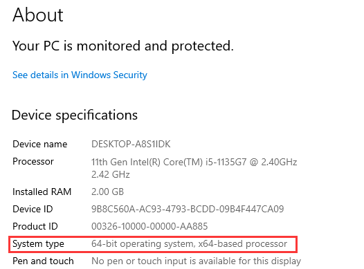
The 64-bit (not 32-bit) version of both Windows and Excel is required, otherwise an exception will occur.
To check whether it is 64-bit:
1 For Windows: Click Settings > System > About to find the information.
2 For Excel: Open Excel and click File > Account > About Excel to get the information on the pop-up dialog, as shown below:
About Microsoft® Excel® 2019 Microsoft® Excel® 2019MSO (Version 2202 Build 16.0.14931.20116) 64Bit Product ID: 00405-32554-86889-AAOEM Session ID: 5DCA85DD-F5BE-4570-8CE4-4D56EF93273D |
About language: Make sure the esProc Desktop version you are installing uses the same language as your operating system. That is, install an English version of esProc Desktop if you are using an English-version of OS, otherwise issues like messy code will occur.
If messy code or other problems occur after an English version of esProc Desktop is installed under an English-version of OS, check OS configurations in Settings > Time & language > Language to make sure the current language selected on Windows display language menu is English.
2 Necessary files
ExcelSpl.xll: The add-in file located in esProcDesk/bin under esProc Desktop installation directory;
scu-Excel-xll-2.10.jar and xll4j-0.0.2.jar: The necessary jar files located in esProcDesk/lib under esProc Desktop installation directory;
ExcelSpl.ini: The configuration file located in esProcDesk/config under esProc Desktop installation directory;
esproc_template.xla: The macro file located in esProcDesk/bin under esProc Desktop installation directory.
3 Load ExcelSpl.xll add-in for Excel
Open Excel, click Options > Add-ins and go to Mange Excel add-ins to have the pop-up Add-ins dialog, where you continue to click Browse to choose the add-in file ExcelSpl.xll. Make sure the new add-in is selected and then restart Excel. Below shows the new add-in after it is successfully loaded:
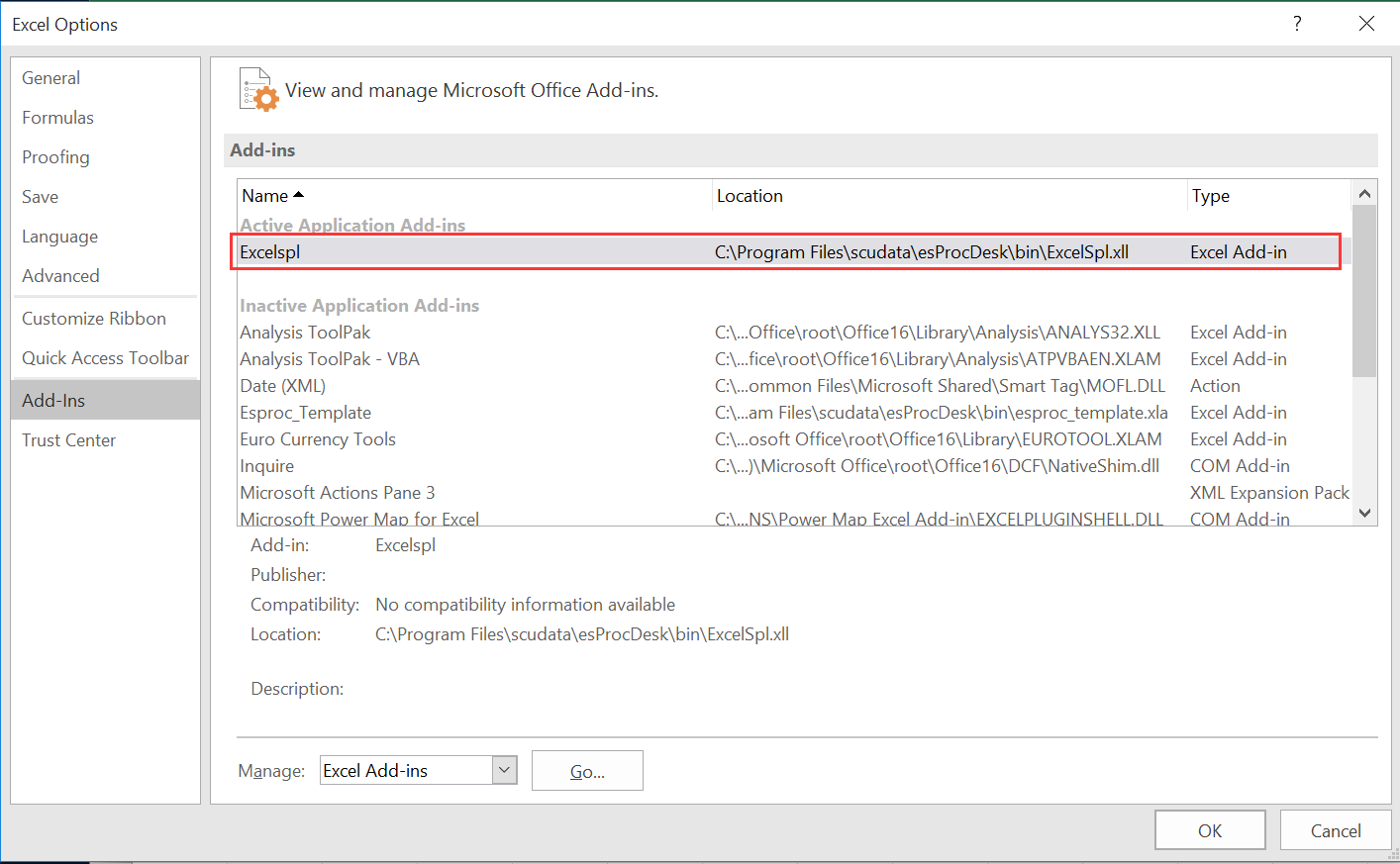
The spl() function will be added to Excel after the add-in file is successfully loaded.
Problems you probably encounter in this phase:
Problem 1:
After you select add-in file ExcelSpl.xll and click OK, the mouse begins to spin forever and refuses to move on to the next step. In this case you can forcibly terminate Excel and restart it.
You will see message “Failed to load XX add-in; do you want to disable it?” after restarting Excel.
Click Yes, and re-load the add-in according to same directions.
Problem 2:
After you select add-in file ExcelSpl.xll and click OK, the mouse begins to spin forever and refuses to move on to the next step. In this case you can forcibly terminate Excel and restart it.
There is no message after restating Excel. But you open the Add-in window and find the add-in has been successfully loaded (the previous screen containing successfully loaded add-in displays).
Problem 3:
After you select add-in file ExcelSpl.xll and click OK, the mouse begins to spin forever and refuses to move on to the next step. In this case you can forcibly terminate Excel and restart it.
There is no message after restarting Excel. When you open the Add-ins window, you find the loading of add-in file failed. Then you repeat the same operations, trying to load the add-in, but fail again by getting stuck at the same point.
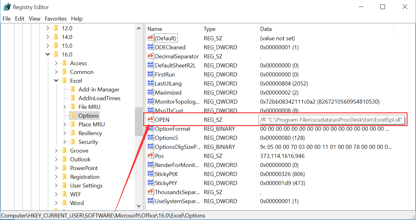
In this case, the solution is to close Excel, open Windows registry, and add the following item.
Note:
1. The value of OPEN item is string /R followed by a string enclosed within the double quotation marks. The content of the latter string is add-in ExcelSpl.xll’s full-path file name;
2. The path under which the registry’s OPEN item is added may vary depending on versions of Excel. It is Computer\HKEY_CURRENT_USER\SOFTWARE\Microsoft\Office\16.0\Excel\Options for Excel2019, and it could be Computer \HKEY_CURRENT_USER\SOFTWARE\Microsoft\Office\15.0\Excel\Options with lower versions. Please find the location according to the Excel version you are using.
Now you open Excel and find that the add-in is listed in the Add-ins window, which means it is successfully loaded.
4 Import macro file for Excel
Find macro file esproc_template.xla in esProcDesk\bin directory under esProc Desktop installation directory and copy it to【Excel installation directy\XLSTART】folder, such as C:\Program Files\Microsoft Office\Office16\XLSTART. The macro file will be automatically imported at the startup of Excel only when it is put under this folder. The import will fail if it is placed in any other folder.
Then, in Excel, click Options > Trust Center > Trust Center Settings > Macro Settings, select Enable all macros, and restart Excel.
Note:
1. Different versions of Excel may have different paths for the startup folder, so make sure you open your Excel, find the correct path, and copy the macro file esproc_template.xla into it.
2. The macro file defines a macro and its hotkey (Ctrl-Enter) to handle multiple return values. The hotkey can be changed if it conflicts with a hotkey that already exists.
3. When spl() function returns a single value, the macro file won’t be used and there is no need to import the macro file.
5 Configure SPL IDE main path
To deploy the SPL IDE main path, the script file (.splx) to be invoked should be placed in the target directory in advance, otherwise the search will fail. To set the main path, follow the directions below:
Open SPL IDE, click Tool > Options, and select Environment to find Main path:
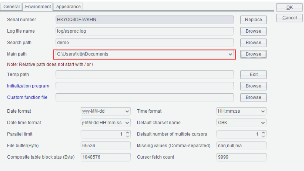
Restart SPL IDE and Excel to make the configuration come into effect.
6 Logs
You can view exceptions in the log file. The file’s path is %appdata%\esproc\tmp\Excel.log.
Ⅱ Using spl() Function in Excel
Once the add-in is installed and configured, the spl() function will be added to Excel for executing a SPL script in a specific Excel cell and obtaining result set.
The spl() function has two syntactic formats:
spl(exp, arg1, …)
Parameters:
exp |
A SPL expression string preceded by =. The question mark is used to represent a parameter. ?1 represents the first parameter, ?2 represents the second one, and so on. |
arg1,… |
Parameter values. There can be none or multiple parameters (30 at most). Parameter values can be constants, or a referenced Excel cell or range of cells. Note: When the Excel add-in cannot identify data types, such as date, datetime and time, of certain parameters, use E() function to perform type conversion. |
In a complex computation, it executes a SPL script file using the following format:
spl(splx(…), … )
Parameters:
splName() |
Script file name without an explicit extension, whose default is .splx followed by parentheses (). Parameters defined in the script correspond to values listed after the comma in sequence. |
arg1,… |
Same as in the previous syntax |
The spl() function can return a single value, a one-dimensional array, or a two-dimensional array.
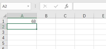
Example 1: No parameters
To generate random integers less than within 100:

Result:
Example 2: A single parameter
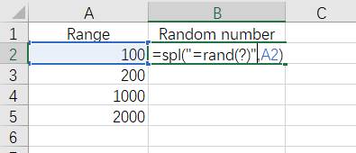
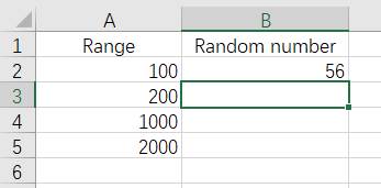
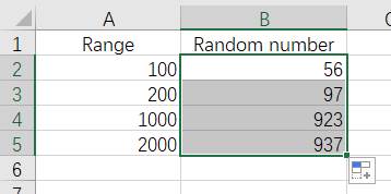
In the following Excel file, the first column contains ranges of random numbers, the second column contains results of generating random integers within the corresponding range:
Result:
Drag B2 down to every relevant cell to obtain all result values:
Example 3: Expression enclosed within double quotation marks
Here’s an Excel file containing date data:
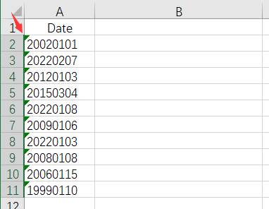
The date data isn’t displayed in any date format due to certain reasons and is recognized by Excel as regular numeric strings (cell type is already set as Text). Now we need to convert them to date type.
SPL has simple solution to this, like =date(A2,"yyyyMMdd"), which parses A2 to date according to the format of "yyyyMMdd". The SPL script itself, however, contains double quotation marks that, when written within the spl() function, need to be escaped according to the Excel escaping rule by writing " as "", as shown below:
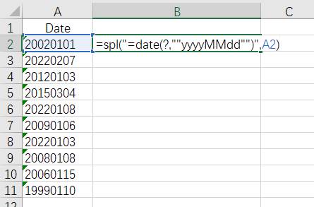
The result is as follows:
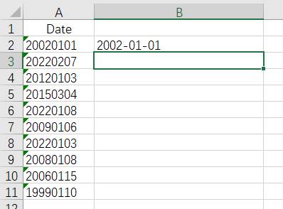
Drag B2 down to every relevanat cell to get the final result:
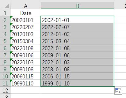
Note:
1. You need to set Cell Type as Text for the cell containing the date data. Select the target cells, right-click to select Format Cells, and under the Number tab, select Text.
2. A green triangle appears at the top left corner when the setting succeeds. If that is not the case, double-click the cells to get into the editing status and shift focus away.
Example 4: Multiple parameters
In the following Excel file, r, g, b, a represent red color, green color, blue color and transparency respectively:
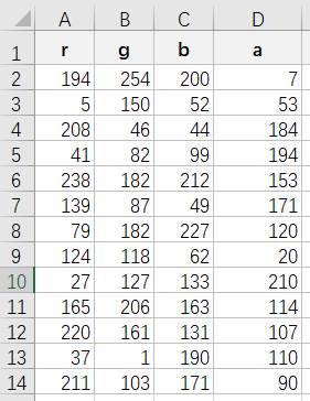
We are trying to add a column on the right to compute the color value combined by proportions of colors for each row. Enter the following SPL code in E2:
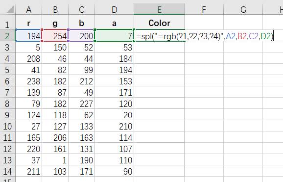
In the code above, ?1,?2,?3,?4 respectivley correspond to the first parameter A2, the second parameter B2, the third parameter C2,f and the fourth parameter D2.
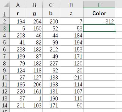
Then we can calcualte the color value for the current row:
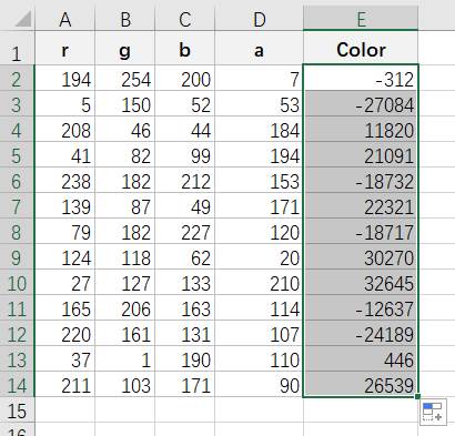
Drag E2 down to every relevant cell:
Example 5: A single-row range parameter
According to the following Excel file, we want to remove the largest value and the smallest value from each row, calculate the median, and insert the result to the column on the right:
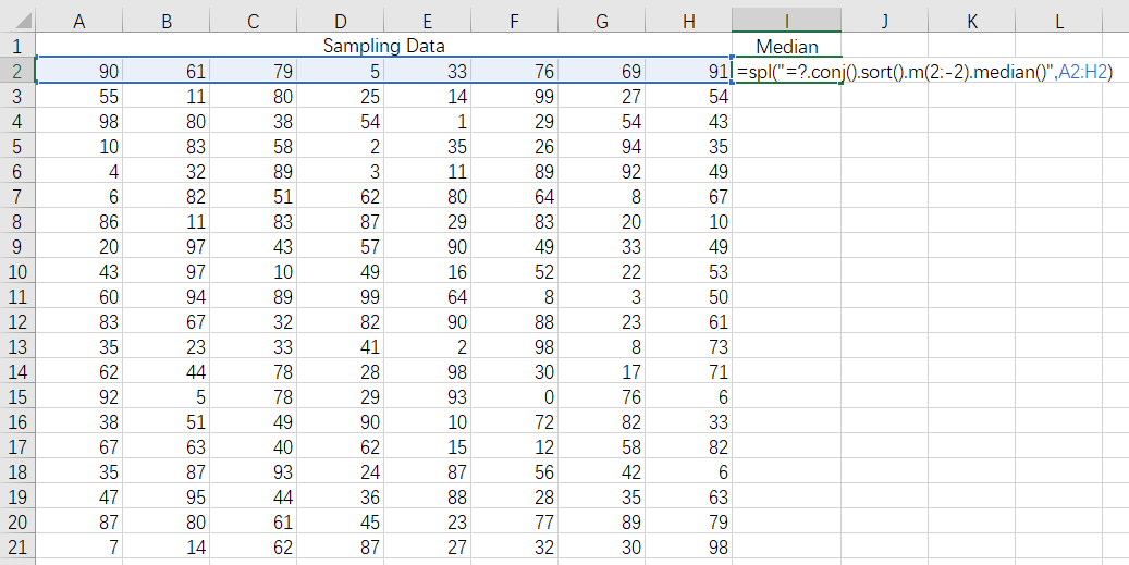
Enter =spl("=?.conj().sort().m(2,-2).median()",A2:H2) in I2. Excel will pass the array combined by the range of cells A2:H2 to SPL expression "=?.conj().sort().m(2,-2).median()" to replace parameter ?, and return the median with the largest and the smallest values excluded. Below is the result:
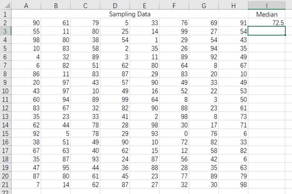
Note: Excel will automatically convert the array parameter to a two-dimensioanl array, even when the array consists of only one row (or one column), and SPL needs to use conj() to assemble a one-level sequence.
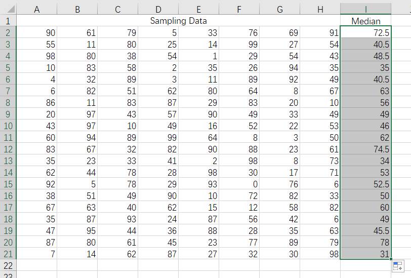
Drag I2 down to every relevant row to automatically compute all medians, as shown blow:
Example 6: A single-column range parameter
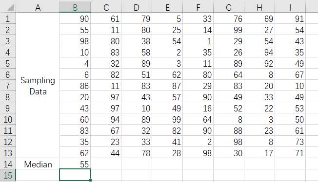
According to the following Excel file, we want to remove the largest value and the smallest value from each column, calculate the median, and insert the result to the row at the end, as shown below:
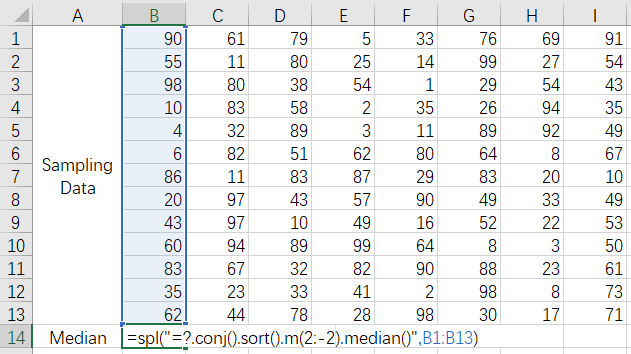
Enter =spl("=?.conj().sort().m(2,-2).median()",B1:B13) in A14. Excel will pass the array combined by the range of cells B1:B13 to SPL expression "=?.conj().sort().m(2,-2).median()" to replace parameter ?, and return the median with the largest and the smallest values excluded. Below is the result:
Note: Excel will automatically convert the array parameter to a two-dimensioanl array, even when the array consists of only one row (or one column), and SPL needs to use conj() to assemble a one-level sequence.
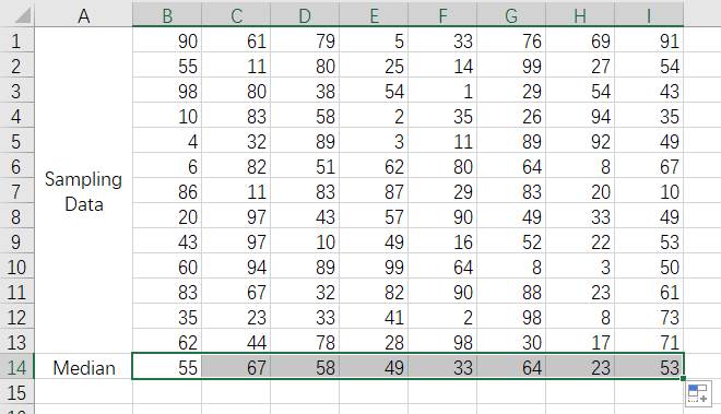
Drag B14 rightward to every relevant column to automatically compute all medians, as shown blow:
Example 7: Multi-row, multi-column range parameter
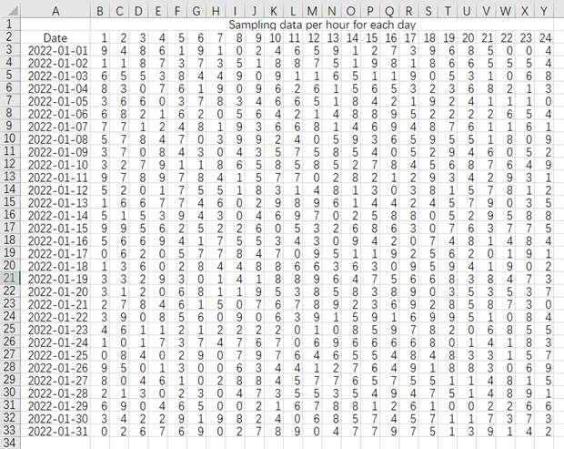
According to the following Excel file:
We want to add a column on the right to hold the cumulative average of sampling data. For the record of the first date, compute the average this one day; for the second record, compute the average of the first two dates; for the third record, compute the average of the first three dates; and so on. Like the above two examples, we remove the largest and the smallest values before we compute each average. Below is the desired result:
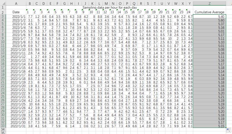
Enter expression =spl("=?.conj().sort().m(2:-2).avg()",$B$3:Y3) in Z3 and get result 5.40. According to the expression, the parameter passed in is $B$3:Y3, where the first cell is preceded by the dollar sign $ because the cumulation always begins from B3 while we copy the expression down to compute each cumulative average.
Drag Z3 down and copy it to every relevant tow to get all cumulative averages.
Example 8: Mixed parameters
The following Excel file records sampling data on the hour per day:
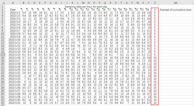
We want to add a column on the right holding average of the largest n values of all samplings by today in the current month. n is determined by the data in column Z.
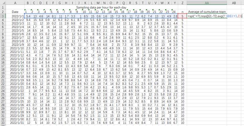
Enter SPL expression =spl("=?1.top@2(-?2).avg()", $B$3:Y3, Z3) in A3.
The first parameter =?1.top@2(-?2).avg() is a SPL formula that gets topn over parameter ?1. n is determined by parameter ?2. Then calculate average of top n values.
The second parameter is $B$3:Y3, which is passed to the SPL formula and corresponds to ?1.
The third parameter is Z3, which is passed to the SPL formula and corresponds to ?2.
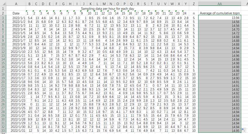
Now drag A3 down to every relevant row to get the final result:
Example 9: Return a one-dimensional array
To generate 10 random integers within 100 and insert them to the first column in sequence:

Enter expression in A1 (as above shows), and press Ctrl-Enter to execute the macro defined in esproc_template.xla and fill result values into a row of cells:
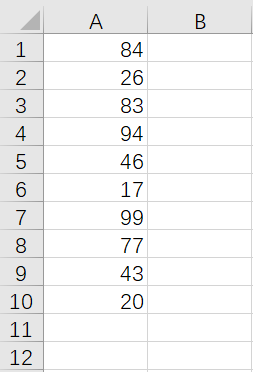
When the expression returns a one-dimensional array, press Ctrl-Enter to fill all members of the array into a column of cells downward beginning from the current cell. Without using this hotkey, only the first member will be inserted to the cell holding the expression.
Example 10: Return a two-dimensional array
We have an Employee.xlsx file:
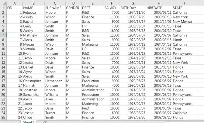
We want to count employees in each department. Enter the SPL script in A1:

It would be the best to put the original Excel file Employee.xlsx under SPL IDE main path. This allows it to be located without the path name, otherwise its full path name should be written explicitly in the expression.
Press Ctrl-Enter to get result:
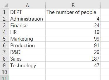
Note:
1. You need to press Ctrl-Enter to trigger the fill action when the expression returns a two-dimensional array. Values will be inserted rightward and downward to a range of cells beginning from the current cell. Only the first member of the array will be filled in the cell holding the expression if the hotkey isn’t used.
2. Escape the double quotation marks ("), if any, in the SPL script by writing it as"" according to the Excel rule.
Example 11: Assemble SPL expression dynamically
We have the following Excel file:
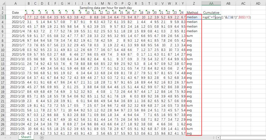
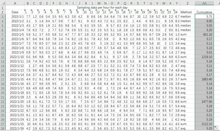
And want to compute the cumulative aggregate of sampling data and insert the results to the column on the right. The aggregate function is specified by the function name given in column Z. When the function name is median, we compute median; when it is avg, we compute the average value; if it is sum, we compute the sum; and so on.
Enter =spl("=?.conj()."&Z3&"()",$B$3:Y3) in A3. In this expression, the first parameter "=?.conj()."&Z3&"()" is a dynamic SPL expression; the second parameter $B$3:Y3 passes an array consisting of values in the range of B3:Y3 to the expression.
In the pass-in parameter $B$3:Y3, the first cell is preceded by the dollar sign $ because the cumulation always begins from B3 and the cell’s value should remain unchanged while we copy the expression down to compute each cumulative aggregate
Drag A3 down to every relevant row to get all cumulative aggregate values.
Ⅲ Editing SPL Script
For certain computations, the SPL expressions may be very complex by consisting of more than one line of code. It is inconvenient to edit the code directly in Excel. In such cases, we can edit the multi-line SPL code in SPL IDE and use Excel Copy/Paste to copy it to Excel for execution.
Example 12: Generate complex SPL scripts in SPL IDE
We have an Excel file as follows:
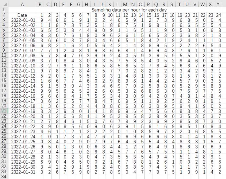
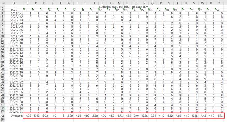
We want to add a row at the end to hold averages of sampling data in each hour in January. We are trying to write one expression to compute all averages on the new row without copying expression for each cell.
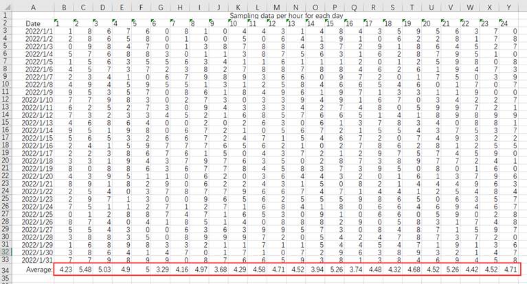
Below is the desired result:
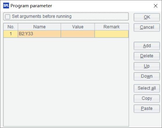
B2:Y33 will be used as the parameter. So, open SPL IDE and define the parameter:
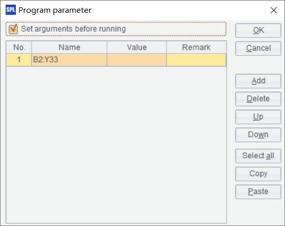
Note: The parameter name must be B2:Y33.
Edit the script:
A |
||
1 |
=E('B2:Y33') |
/ Convert the two-dimensional array parameter 'B2:Y33' to a table sequence, using the first row as column headers; as parameter and cells have same names, enclose the parameter with single quotation marks to distinguish them from each other |
2 |
=to(24).("avg('"+string(~)+"'):'"+string(~)+"'") |
/ Since column names are 1-24, dynamically assemble the aggregate expression for all the 24 columns for simplifying the code |
3 |
=A1.groups(;${A2.concat@c()}) |
/ Place the aggregate expression in groups function to compute averages in all fields |
4 |
return A3(1).array() |
/ Convert result records to a single-level sequence and return it |
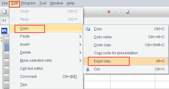
Click Edit > Copy > Excel Copy to copy the SPL script to the clipboard.
Move back to the Excel file, select B34, and press Ctrl-V to copy and paste the SPL code in:
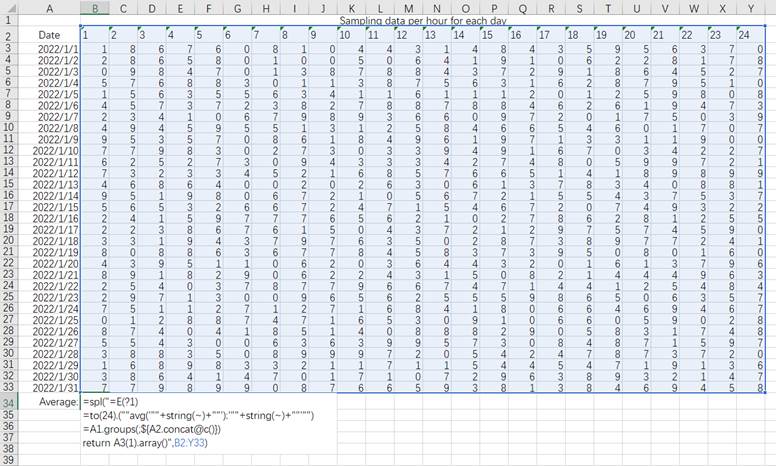
The SPL code returns a one-dimensional array. Remember to press Ctrl-Enter after you enter the expression in to insert values of the returned array into a row of cells from left to right. Below is the final result:
Note:
1. When the SPL script returns a one-dimensional array, the expansion mode is by default the vertical. In Excel, click【Add-ins】-【SPL】-【Show Setting…】and select expansion mode 【Horizontal display】. If this expansion mode option isn’t checked, use vertical display. Then press Ctrl-Enter to insert values of the result set into cells downward for vertical display and from left to right for horizontal display.
2. When a parameter passed to the SPL script is a range of cells (a single row, a single column, or multi-row & multi-column), the parameter value will automatically form a two-level sequence, which can be converted to a table sequence in the SPL script using E() function.
3. The rule for parameters is the same as that for a one-line script. Just use ?1 to represent the first parameter, ?2 to represent the second, and so on.
Example 13: Modify SPL script in SPL IDE
Sometimes we have closed SPL IDE after copying an SPL script to Excel without retaining the code in it. It is inconvenient to modify the code directly in Excel. SPL IDE offers Excel Paste feature to let you copy an SPL script back to SPL IDE for re-editing. The operation is like this:
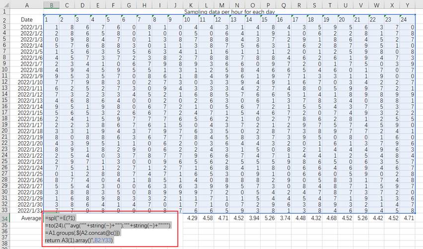
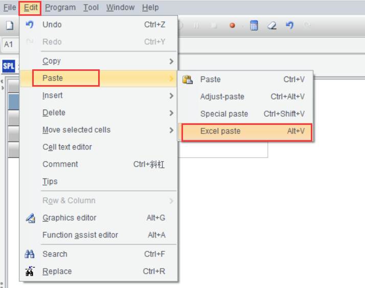
Select the whole SPL code in Excel, press Ctrl-C to copy it to the clipboard. Open SPL IDE and click Edit > Paste > Paste code to restore the original code in SPL IDE, as shown below:

Example 14: Edit extremely long SPL script
We have an Employee.xlsx file as follows (the file should be placed in SPL IDE main path in advance):
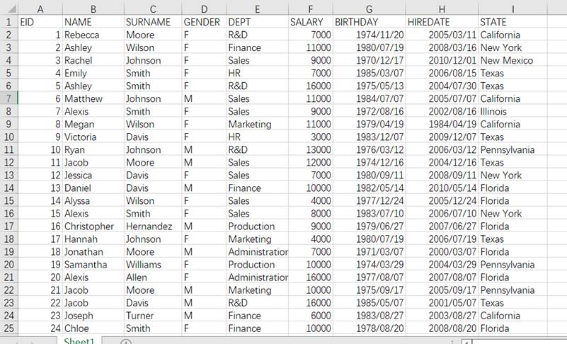
We want to query the file according to a certain condition to get a result set containing only some of the original fields. They are EID, NAME, GENDER, DEPT, SALARY, BIRTHDAY, HIREDATE and STATE. Below shows the query condition:
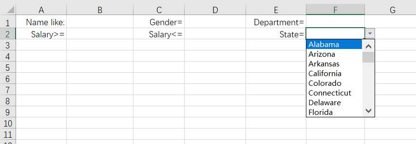
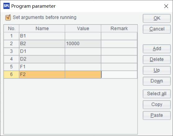
The parameters to be passed to the SPL script are B1, B2, D1, D2, F1, F2.
First, open SPL IDE to define parameters:
Write the following script:

Click Edit > Copy > Excel Copy to copy the multi-line code to clipboard.

Open Excel, select A4, and press Ctrl-V to paste the code in:

Excel has restriction on the length of string in an expression, and will divide an extremely long code into multiple parts after the code is copied to Excel, with each part not longer than 240 characters. If a part of code ends with a slash \, the script goes on and the next parameter is still the code.
Now press Ctrl-Enter to get the final result:

Example 15: Invoke SPL script directly
We can also invoke a long SPL script directly in the spl() function. Take the example in the previous section, we store the SPL script as Example15.splx in SPL IDE main path and enter the following expression in Excel’s A4:

According to the expression, the syntax for invoking the script file direclty is =spl("script file name (?n……)",parameter n….). Write the same number of question marks for parameters in the script, like ?1 representing the first parameter, ?2 representing the second, and so on. The rule is the same as that for writing code directly or that for passing parameters in.
Now press Ctrl-Enter to get the final result:

SPL Official Website 👉 https://www.scudata.com
SPL Feedback and Help 👉 https://www.reddit.com/r/esProc_Desktop/
SPL Learning Material 👉 https://c.scudata.com
Discord 👉 https://discord.gg/2bkGwqTj
Youtube 👉 https://www.youtube.com/@esProcDesktop
Linkedin Group 👉 https://www.linkedin.com/groups/14419406/


Chinese version