

Pre-calculating mechanism of SPL
Partial pre-aggregation
The backend operation of the multi-dimensional analysis is essentially the grouping and aggregating, which can be performed directly on the data. However, when the amount of data is very large, it is difficult to achieve an instant response.
To solve this problem, an easy way to think of is the pre-aggregation, that is, calculate every aggregation result in advance and save them as an intermediate result (we will hereinafter call it cube). When the front-end application requests, we can directly search the cube and return the result.
For example, pre-aggregate the order table in Figure 1 below:

Figure 1 Pre-aggregating order table
In this figure, the order table is combined into 22=4 cubes by the two dimension: data and department, and each cube will calculate the pre-aggregated value of the amount such as the sum, average and count, etc. The 4 cubes contain all combinations of the two dimensions, we call it full pre-aggregation.
Pre-aggregation is actually to trade space for time. In other words, although the cube occupies more storage space, it turns the traversal problem to a search problem, and hence the instant response can be achieved theoretically.
For example: to calculate the total order amount of the department 20 on Jan. 1, 2016, directly searching cube4 will work; to count the order amount, average, etc. by date, we only need to read cube3.
However, the full pre-aggregation is basically infeasible in practice, and a simple calculation will show you why.
When performing the full pre-aggregation for 50 dimensions, 250 cubes will be required, and at a conservative estimate, the required volume will be over one million terabytes, therefore, it is inoperable. Even if only 10 dimensions are pre-aggregated (10 dimensions are not large in number since both the grouping and slicing dimensions are included), it still requires at least hundreds of terabytes of storage space, and hence the practicality is very poor.
SPL provides the partial pre-aggregation mechanism, which only pre-aggregate part of combinations of dimensions. When the front-end requests, first search for the pre-aggregated data under a certain condition, and then do the aggregation. For the order table mentioned above, partial pre-aggregation can use the scheme shown in Figure 2 below:
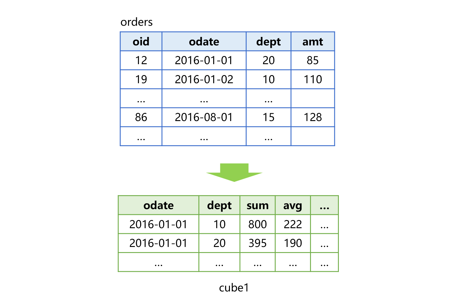
Figure 2 Partial pre-aggregation of order table
In this figure, only one cube (cube1) is generated in advance. If you want to calculate amount of order on 2016-01-01 for the department 20, directly searching cube1 will work. However, when counting the order amount and average value by date, it needs to do another grouping and aggregating by date based on cube1.
Compared with full pre-aggregation, the storage space occupied by partial pre-aggregation is greatly reduced, but the performance can be improved by dozens of times on average, and it can often meet the requirements.
In practice, SPL can create multiple pre-aggregated cubes as needed. For example, the data table T has five dimensions A, B, C, D and E. According to business experience, we calculate several most commonly used cubes in advance, as shown in Figure 3 below:
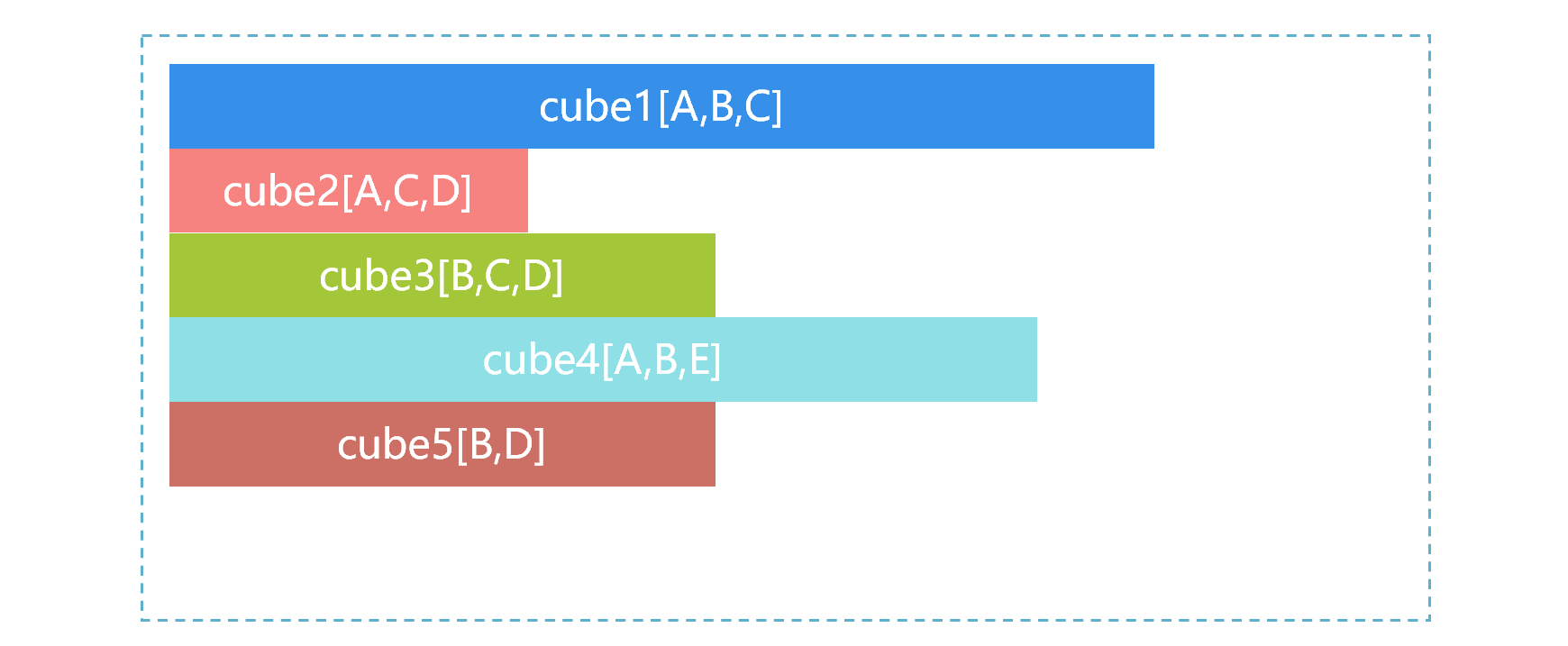
Figure 3 Multiple pre-aggregated cubes
In Figure 3, the size of the storage space occupied by the cube is represented by the length of the bar, cube1 is the largest, and cube2 is the smallest.
When the front-end application sends a request for statistical aggregation that needs to be made according to B and C, SPL will automatically select from multiple cubes, and the process is roughly as shown in Figure 4 below:
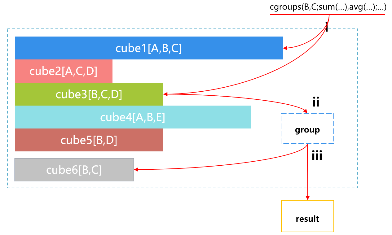
Figure 4 Selecting by SPL from multiple cubes
Step i, SPL will automatically find the available cubes, which are cube1 and cube3. Step ii, when SPL finds that cube1 is relatively large, it will automatically select the smaller cube3, and do the grouping and aggregating by B and C based on cube3. Step iii, return the results.
If the returned results are saved, such results can be used directly when grouping and aggregating by B and C is requested again in the future. However, since SPL cannot judge whether such results need to be saved, the programmers should judge and do it themselves. Similarly, programmers can also implement other engineering means by themselves, such as performing the statistical analysis following the record of the historical query requests and deleting the infrequently used cubes in a timely manner.
SPL code for pre-calculating cube is roughly as follows:
A |
|
1 |
=file("T.ctx").open() |
2 |
=A1.cuboid(file("1.cube"),A,B,C;sum(…),avg(…),…) |
3 |
=A1.cuboid(file("2.cube"),A,C,D;sum(…),avg(…),…) |
… |
Using the cuboid function can create the pre-aggregation data. You need to specify the pre-aggregation data file name, and the remaining parameters are the same as that of grouping and aggregating algorithm.
It is also very simple to use:
A |
|
1 |
=file("T.ctx").open() |
2 |
=A1.cgroups(B,C;sum(…), avg(…) ;file("1.cube"), file("2.cube"),…) |
The cgroups function will automatically search for the most appropriate pre-aggregated data according to the above logic before calculation.
Although the pre-aggregation scheme is quite simple, since it is limited by the storage volume, there are many limitations in practice, as a result, it can only deal with the most common situations.
Time period pre-aggregation
For the counting on the time period, SPL provides a special time period pre-aggregation mechanism.
For example, for the order table, there is already one cube (cube1) pre-aggregated by date odate, then we can add one cube (cube2) pre-aggregated by month, as shown in Figure 5 below:
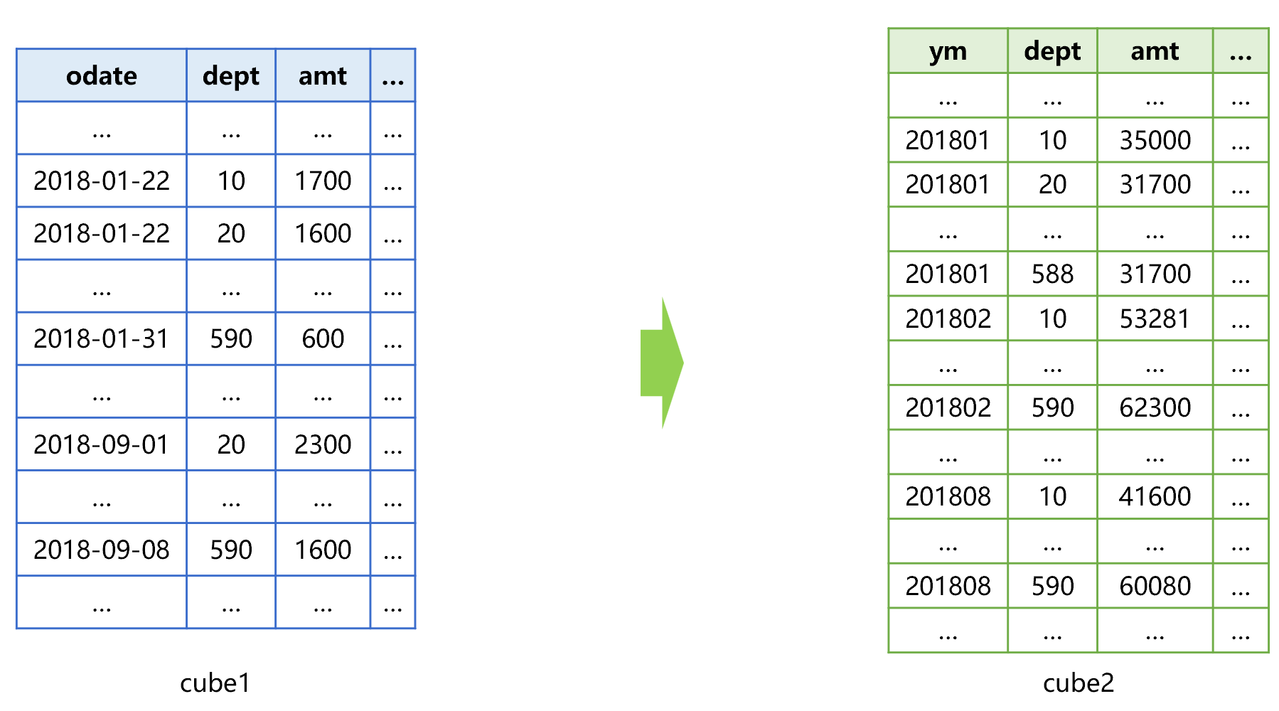
Figure 5 Adding one cube (cube2) pre-aggregated by month
Not only can SPL use the cube2 to speed up the aggregation by month, but also perform more fine-grained time interval aggregation. For example, when we want to calculate the total amount from Jan. 22 to Sept. 8, 2018 based on the group by department, the approximate process is shown in Figure 6 below:
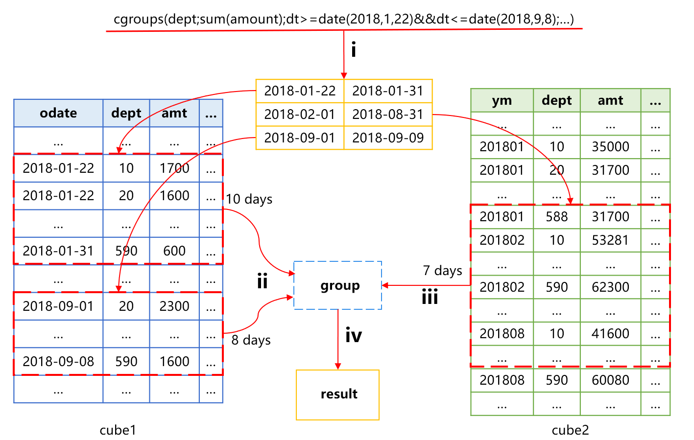
Figure 6 Pre-aggregation mechanism for time period
Action i in Figure 6 is to divide the time into three segments. Segment 1 is the first 10 days, segment 2 is the middle 7 whole months, and segment 3 is the final 8 days.
Action ii is to use cube1 to calculate the aggregated value of segments 1 and 3, including the data of 18 days. We assume that the average number of departments included in each day is m, then the amount of data involved is 18*m records.
Action iii is to use cube2 to calculate the aggregated value of segments 2, including the data of 7 whole months. The average number of records per whole month should also be close to m, and the amount of calculation involved is 7*m records.
Action iv is to do grouping and aggregating again based on the obtained results.
In this way, the total calculation amount involved is 18*m+7*m=25*m. If that cube1 was used to aggregate directly, the calculation amount from Jan. 22 to Sept. 8 would be 223*m records. Therefore, using the time period pre-aggregation mechanism can reduce the calculation amount by almost 10 times.
SPL code that implements the above mechanism is roughly as follows:
A |
|
1 |
=file("orders.ctx").open() |
2 |
=A1.cuboid(file("day.cube"),odate,dept;sum(amt)) |
3 |
=A1.cuboid(file("month.cube"),month@y(odate),dept;sum(amt)) |
4 |
=A1.cgroups(dept;sum(amt);odate>=date(2018,1,22)&&dt<=date(2018,9,8);file("day.cube"),file("month.cube")) |
The cgroups function adds the condition parameter. When SPL finds there are time period condition and higher-level pre-aggregated data, it will use this mechanism to reduce the amount of calculation. In this example, SPL will read the corresponding data from pre-aggregation files month.cube and day.cube respectively before aggregation.
Redundant sorting
The aggregation operation without any slice filtering condition will involve all data. If a suitable cube can't be found, there is no way to reduce the amount of calculation. However, when there is the filtering condition, if the data are reasonably organized, we can find ways to avoid traversing all data even if there is no suitable cube.
One simply way is to create the index on the dimensions, which will work, but just a little. Although the index can quickly locate the records that meet the condition, if the physical storage locations of the records are not continuous, there will still waste a lot of time while reading. When the target data are too scattered, it may not be much better than full traversal. The reason is that in multidimensional analysis operation, the amount of data to read is still very large even if slicing is performed. The main application scenario of index is often to select a small amount of data.
If the data are stored orderly by a certain dimension, the slicing condition of this dimension can be used to limit the target data in a continuous storage area, in this way, there is no need to traverse all data, and the amount of reading can be effectively reduced. However, each dimension may have a slicing condition in theory, if the data are sorted by each dimension, they will be copied several times, as a result, the storage cost is somewhat high.
SPL provides a redundant sorting mechanism, which can not only reduce the occupied storage space, but also avoid traversing all data. For example, the table T has 10 dimensions, and SPL uses two ways to sort and store them, roughly as shown in Figure 7 below:
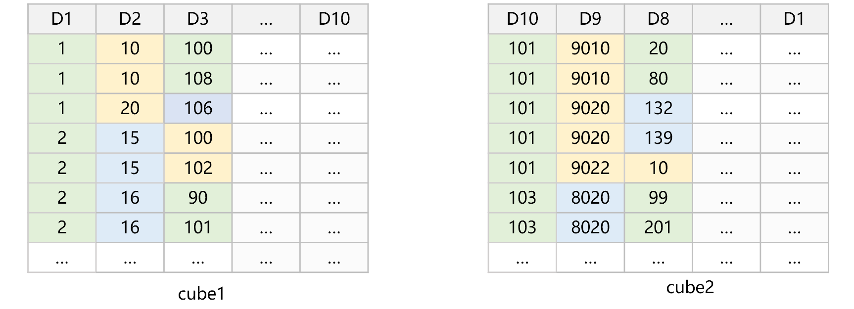
Figure 7 Redundant sorting
In this figure, the dimensions are sorted and stored as cube1 according to the order of D1, D2,..., D10, and then sorted and stored as cube2 according to the order of D10, D9,..., D1. In the two cubes, the closer to the front the position of dimension in the sorted dimension list, the higher the degree of physical order of data after filtering will be. For example, D10 in cube2 is at the front, the data can be concatenated into a large area after filtering; while for D9 and D8, since their positions are relatively close to the front, although the data after filtering cannot concatenated into a large area, but they are also composed of some relatively large continuous areas.
For any dimension D, there will always be a data set that can make D be in the first half of its sorted dimension list. For example, when we want to do the slice filtering to D7, SPL will automatically select cube2 since it finds that D7 is closer to the front of the sorted dimension table of cube2.
When multiple dimensions have slicing conditions, SPL will choose the dimension whose value range is smaller than the total value range after slicing, which makes the amount of filtered data smaller.
For example, D8, D6 and D4 all need to be sliced, SPL will select the slicing condition of D8 to filter since it finds D8 is at the front of the sorted dimension table of cube2, while the conditions of D6 and D4 will still be calculated during traversal. The reason is that in multidimensional analysis, the slice on a certain dimension can often reduce the amount of data involved by several times or tens of times. It will be of little significance to reuse the slicing condition on other dimensions, and it is also very difficult to implement.
SPL code for implementing redundant sorting is roughly as follows:
A |
|
1 |
=file("T.ctx").open() |
2 |
=A1.cuboid(file("1.cube"),D1,D2,…,D10;sum(…)) |
3 |
=A1.cuboid(file("2.cube"),D10,D9,…,D1;sum(…)) |
4 |
=A1.cgroups(D2;sum(…);D6>=230 && D6<=910 && D8>=100 && D8<=10 &&…; file("1.cube"), file("2.cube")) |
In A2 and A3, cuboid will create different pre-aggregated data for different dimension order.
The redundant sorting mechanism is implemented in the cgroups function. If it is found that there are multiple pre-aggregated data sorted by different dimension and there is slicing condition, the most appropriate pre-aggregated data will be selected.
We can also manually select a properly sorted data set with SPL code, and store more sorted data sets.
The redundant sorting method is not only appropriate for multidimensional analysis, but also for the conventional traversal with filter conditions.
SPL Official Website 👉 http://www.scudata.com
SPL Feedback and Help 👉 https://www.reddit.com/r/esProc
SPL Learning Material 👉 http://c.scudata.com
SPL Source Code and Package 👉 https://github.com/SPLWare/esProc
Discord 👉 https://discord.gg/ydhVnFH9
Youtube 👉 https://www.youtube.com/@esProc_SPL


Chinese version