

SPL Pseudo Table Bi-dimension Ordering Mechanism
Performing statistical analysis based on detail user/account data is a common computing scenario, covering computing goals from user behavior analysis, bank account analytics, calculating funnel conversion rate to insurance policy analysis, and so on. We call all of them account analysis. The scenario has certain characteristics – a huge volume of total data versus a small amount of data in each account; long total time span versus short time for each computation; and no exchanges between accounts versus probably complicated computations within one account.
Generally, this type of computing scenario involves filtering on time dimension. If data can be ordered and stored by time in advance, a large amount of data that does not meet a specified time condition can be first filtered away, considerably speeding up the filtering operation. As the subsequent computations will be performed by account, ordering data by account also facilitates the filtering, makes coding easy and increases performance.
But one data table cannot be ordered by two dimensions at the same time. Even if there are two sorting fields, they need to be used one by one. Sorting data first by account results in unordered time points and makes it impossible to exclude useless data quickly. Putting time first enables to filter data quickly by time but gets a result set unordered by account. When the available memory space is enough, it is beneficial to sort data first by time and then by account. The result of filtering by time can be wholly loaded into the memory and computed fast using the memory’s performance advantages. Yet, if the filtering result set is still huge and needs to be computed outside the memory, the performance will be bad.
SPL pseudo tables support bi-dimension ordering mechanism that enables data to be ordered by the time dimension on the whole (which helps to achieve fast filtering) while keeping filtering result set ordered by account (which facilitates subsequent computations). This makes it appear that data is ordered by two dimensions at the same time.
Storage structure and data retrieval process
A pseudo table is an object defined on a multi-zone composite table . A multi-zone composite table consists of multiple composite tables of same structure. Each of these composite tables is a zone table .
Suppose multi-zone composite tableTstores detail account transaction data in multiple fields including user account (userid), date (dt), city the account belongs to (city), product (product) and transaction amount (amt), etc. The multi-zone composite table has 12 zone tables that store data of the 12 months in order, as the following shows:

Figure 1 Multi-zone composite tableT.ctx
As the figure shows, zone tables are ordered by dt as a whole. And data in each zone table is ordered by userid and dt. Take the second zone table2.T.ctxas an example, its data is arranged as follows:
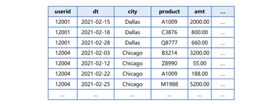
Figure 2 Zone table2.T.ctx
With a multi-zone composite table, we can define a pseudo table using a structure made up of definite name attributes (which can also be regarded as a record whose fields are the attributes), as the following shows:

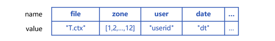
Figure 3 Pseudo tableT’s attributes and their values
Attribute file is name of the multi-zone composite table from which the pseudo table is generated (here it isT.ctx); zone represents the zone numbers, which, in this case, is a set containing numbers from 1 to 12, in the multi-zone composite table; date is name of the time dimension field, which is "dt". As zone tables in the multi-zone composite table are separated according to the time dimension field, we call the field zone expression .
A pseudo table will compute and record the maximum and the minimum zone expression values (dt field values) for each zone table, as shown below:
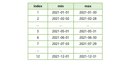
Figure 4 A set of max/min zone expression values
The row of index 2 shows that in zone table 2’s data the minimum dt value is 2021-02-02 and the maximum data value is 2021-02-28. Make a note that multi-zone composite tableT.ctx, at its creation, should use userid and dt as its dimensions. This, on the one hand, can ensure that both userid and dt are ordered in each zone table, and on the other hand, avoid full table traversal for getting the set of max/min zone expression values in an effort to generate the pseudo table faster as the max/min dimension values are already stored in the composite table.
Now let’s look at how to retrieve data from a pseudo table. Suppose we are trying to get data whose dt field values are between 2021-05-15 and 2021-05-25 and group and compute data by userid.
First, SPL can recognize that filtering condition dt is pseudo tableT’s zone expression. Then it will match the set of max/min zone expression values using the start and end dt time points specified in the filtering condition. The result is as follows:
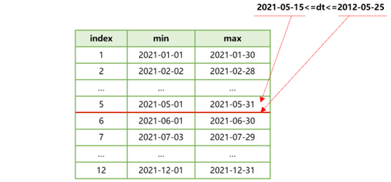
Figure 5 Match the set of max/min zone expression values
According to Figure 5, the filtering condition is within the range of max/min zone expression values corresponding to zone table 5. This means that data meeting the dt filtering condition is stored in zone table 5 of multi-zone composite tableT.ctx. Now we can just filter all the other zone tables and only retrieve zone table 5 for the subsequent computations.
Since data in each zone table is already ordered by userid and dt, SPL will retrieve data from zone table 5 in batches in order for the subsequent order-based grouping operation.
As zone table 5 is not ordered by dt, filtering on dt by the filtering condition is needed at retrieval. Though this involves traversal of the zone table, it is still much faster than full traversal of the multi-zone composite table.
Now we expand the time span of the filtering condition to 2021-07-05 and the SPL process of finding the set of max/min zone expression values will be as follows:
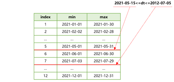
Figure 6 Match the set of max/min zone expression values
In this case, data meeting the dt filtering condition falls in three continuous zone tables – 5, 6 and 7. As the three tables are ordered by userid, SPL, in the next-step computation, will merge them by userid when retrieving data in batches through cursor, making preparation for the subsequent order-based grouping.
Here the traversal covers the three zone tables.
Below is the SPL code of generating the pseudo code and retrieving data from it:
A |
|
1 |
=create(file,zone,date).record(["T.ctx",to(12),"dt"]) |
2 |
>T=pseudo(A1,0) |
3 |
=T.select(dt>=date("2021-05-15") && dt<= date("2021-07-05") ) |
4 |
=A3.groups@u(userid;...) |
A1 prepares the pseudo table definition according to the specified attributes.
A2 generates a pseudo table object. Pseudo tables support multithreaded processing. Here pseudo function’s second parameter is 0, meaning that the system default number of threads will be used.
A3 quickly filters pseudo tableTby the time dimension. In A4, groups function performs an order-based grouping on the filtered pseudo table.
If the computation by each userid is too complicated, we can retrieve data by userid and implement computations through multi-step code:
A |
B |
|
… |
… |
|
4 |
=A3.cursor() |
|
5 |
for A4;userid |
… |
A4 defines a cursor on the filtered pseudo table. A5 fetches data of one userid each time from the cursor for complex computation. And this goes on by loop.
Application examples
We will perform a few more complicated computing tasks based on the above data. With the result set of filtering pseudo tableTby time dimension, we need to group it by product and in each group count all unique userids and sum amounts. SPL does the job using the following code:
A |
|
1 |
=T.select(dt>=date("2021-05-15") && dt<= date("2021-07-05") ) |
2 |
=A1.groups@u(product;icount(userid),sum(amt)) |
A1 performs fast filtering on pseudo tableTby the time dimension. A2 performs order-based grouping on A1’s result, and then count distinct and sum.
As A1’s result set is ordered by account (userid), SPL automatically uses order-based count distinct algorithm. This is much faster than a case where userid is unordered and needs small memory space.
There are more complex scenarios, such as calculating funnel conversion rate for an E-business. Suppose account transaction event tableT1consists of fields account (userid), transaction time (etime) and event type (etype). The etype could be "login", "search", "pageview" or others. A typical funnel conversion rate calculation is to find the number of accounts that perform a series of continuous events like login, search and pageview within a specified time period. The later the events happen, the fewer the number of accounts that reach them. The frequencies of events is like a funnel that has wide top and narrow bottom.
To handle this scenario, we need to retrieve account data from the pseudo table in loop and compute it using multi-step code according to the time order. SPL generates the following code:
A |
B |
C |
D |
|
1 |
=["login","search","pageview"] |
=A1.(0) |
||
2 |
=T1.select(dt>=date("2021-05-15") && dt<= date("2021-06-14")).cursor() |
|||
3 |
for A2;userid |
=first=A3.select(etype==A1(1)) |
if first.len()==0 |
next |
4 |
=t=null |
=A1.(null) |
||
5 |
for A1 |
if #B5==1 |
>C4(1)=t=t1=first.dt |
|
6 |
else |
>C4(#B5)=t=if(t,A3.select@1(etype==B5 && dt>t && dt<elapse(t1,7)).dt,null) |
||
7 |
=C4.(if(~==null,0,1)) |
>C1=C1++B7 |
||
A2 defines a cursor based on the fast filtered pseudo table. A3 fetches data of one account each time for complicated computation.
Since one user’s all data can be quickly fetched in each round of loop, only a few lines of code are needed to accomplish the complicated funnel conversation rate calculation. Find more discussions about the calculation in SQL Performance Enhancement: Conversion Funnel Analysis , which introduces ways of making the code even shorter.
SPL Official Website 👉 http://www.scudata.com
SPL Feedback and Help 👉 https://www.reddit.com/r/esProc
SPL Learning Material 👉 http://c.scudata.com
SPL Source Code and Package 👉 https://github.com/SPLWare/esProc
Discord 👉 https://discord.gg/ydhVnFH9
Youtube 👉 https://www.youtube.com/@esProc_SPL


Chinese version