SPL Pseudo Table Data Type Optimization

A table storing data physically (which is simply called physical table) usually uses some storage mechanisms to boost performance and reduce space usage.

But they usually lead to lower data readability and higher coding complexity. For example, using integers to represent enumerated values or using bits of integer field to store boolean values. Integers and binary digits are not as easy to read as strings and booleans. And we need to write code for type conversion and binary computation over these physical values.

A SPL pseudo table is a logical table defined on a physical table. We can define easier to use logical fields in a pseudo table. Such logical fields are called pseudo fields, and fields that physically exist in the physical table are called real fields.

Through mapping between the pseudo fields and the real fields, a pseudo table encapsulates the special storage structure and achieves transparent storage mechanism for the physical table. This helps reduce hard disk usage and increase performance, as well as making data easier to read and handle.

Following illustrates how to use different types of pseudo fields in a pseudo table.

Enumerated dimension

In real-world practices, the value ranges of many enumerated fields are a set of strings. Integers are usually used in physical tables to represent strings. They occupy less space and compute faster than strings, but they are harder to understand and handle.

Storing both strings and numbers can obtain good performance and ease-of-use at the same time. But this also increases time spent in generating data and disk usage, even could cause the error that strings and numbers are not consistent.

Below is structure of a physical table storing transaction details:

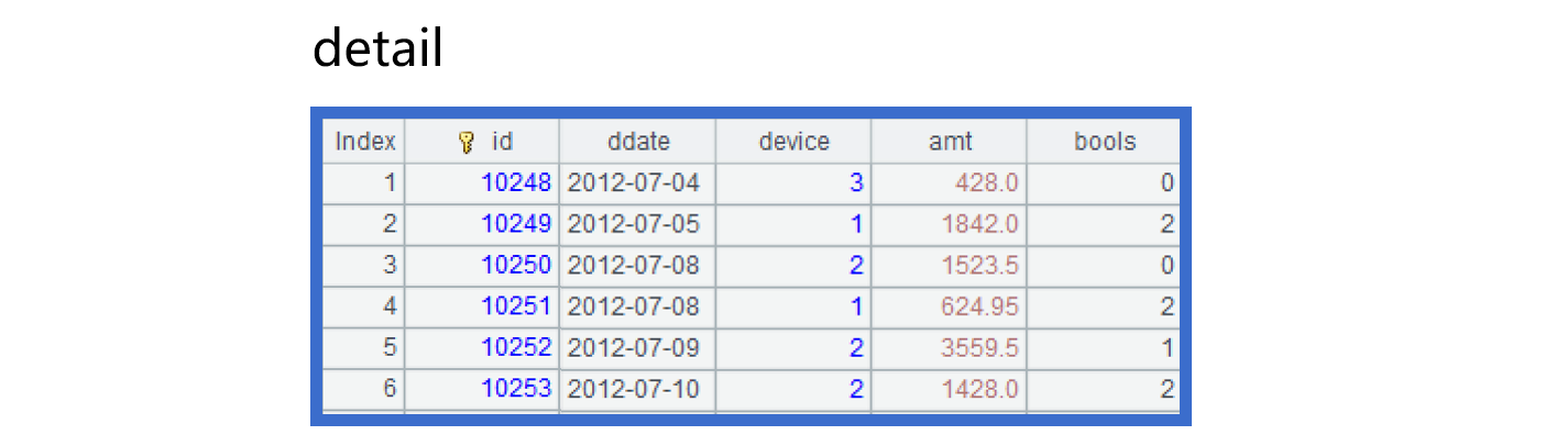
In the above detail table, the enumerated field device stores integers 1, 2 and 3, which corresponds to three types of devices – computer, smart phone, and pad. The task is to filter data according to whether the device used in transactions is smart phone or pad, group data by transaction date (year and month) and device, sum amounts and calculate the number of transactions in each group, and display the result set as easy to read strings.

We can handle such a scenario through the pseudo table’s enumerated dimension – using a pseudo field to define the mapping relationship between numbers and strings.

By defining an enumerated dimension, we can directly use strings in a computing expression and get strings in the result set while still storing numeric values in the physical table to achieve high performance.

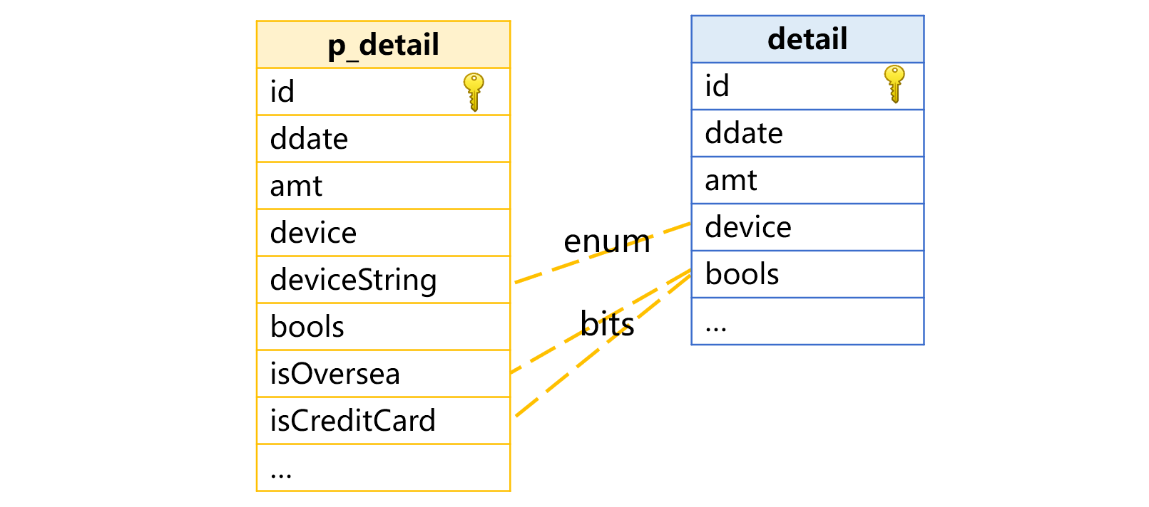
In the picture below, a pseudo field deviceString is defined for pseudo table p_detail to make transparent enumerated dimension:

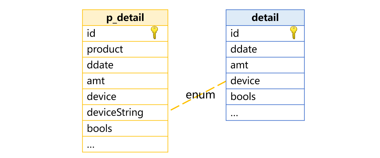
The physical table detail does not have a deviceString field. The field needs to be obtained by converting the enumerated set list, which is [“computer”,“smart phone”,“pad”] in this example. The three enumerated values correspond to natural numbers 1, 2 and 3 respectively.

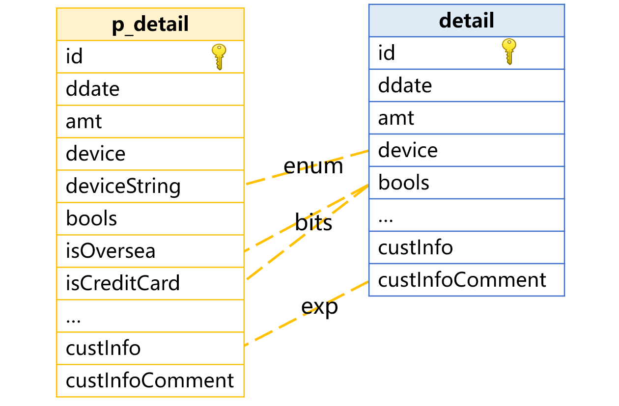
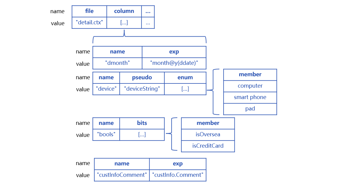
SPL uses a multi-attribute structure to define a pseudo table. Each attribute has a fixed name. In this instance, pseudo table p_detail’s definition contains physical table name, enumerated dimension (enum) name and list set, as shown below:

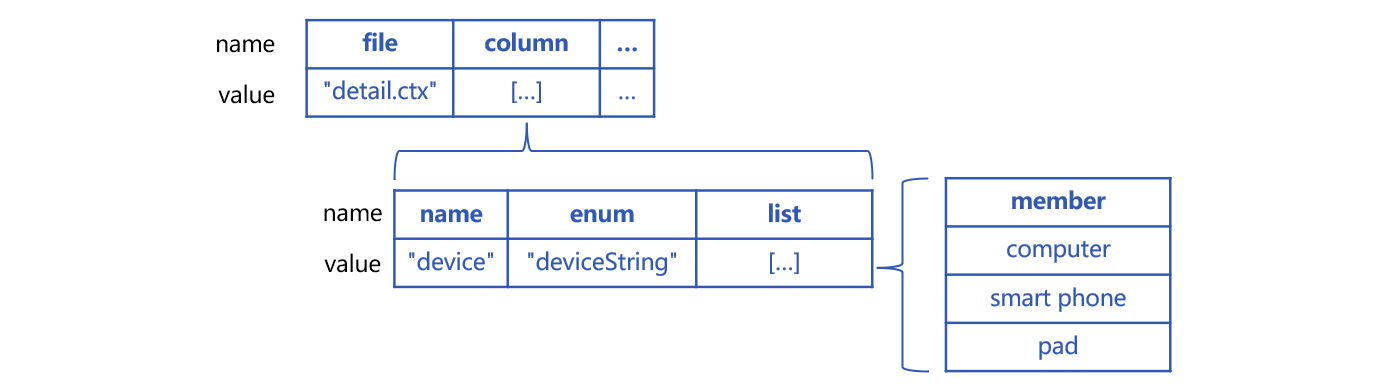
Attribute file is the physical table name based on which the pseudo table is generated. Its value is composite table “detail.ctx”. Attribute column commands a set of special fields. Each of its members corresponds to a special field. name is the real field name “device”. enum defines the pseudo field name “deviceString”. The set of enumerated values under list is [“computer”,“smart phone”,“pad”].

Below is the SPL code for defining pseudo table p_detail:

	A
1	=[{file:“detail.ctx”, column:[ {name:“device”,enum:“deviceString”,list:[“computer”,“smart phone”,“pad”]} ] }]
2	>p_detail=pseudo(A1)

A1 prepares the pseudo table structure, which includes an enumerated type pseudo field deviceString.

A2 generates pseudo table p_detail.

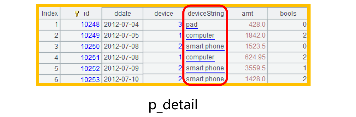
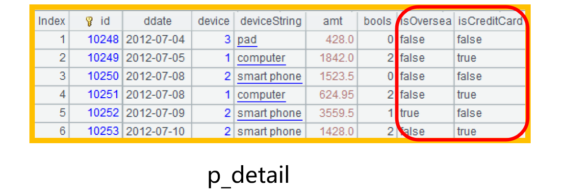
After the pseudo table is generated, we use cursor p_detail.cursor(id,ddate,device,deviceString,amt,bools).fetch(6) to retrieve some data from it, as shown below:

Regard p_detail as a simple data table and directly use deviceString field to perform the conditional filtering and grouping:

	A
	…
3	=p_detail.select(deviceString==“pad” || deviceString==“smart phone”)
4	=A3.groups(month@y(ddate):dmonth,deviceString;sum(amt),count(~))

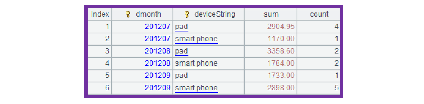
A3: Strings “smart phone” and “pad” in the filter condition are first automatically converted to 2 and 3 respectively and then used to filter physical table detail.

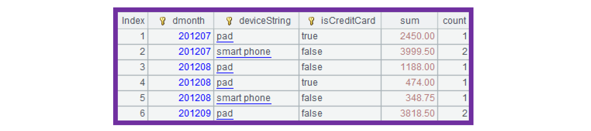
A4: The device field values 2 and 3 are transformed back to “smart phone” and “pad” respectively for the result set, as shown below:

Updating a pseudo table (update) or appending data to it (append) will actually change the corresponding physical table.

For a pseudo table having an enumerated dimension, it is OK to only have pseudo field values for appending or modifying data because SPL can automatically convert them to corresponding real field values.

For the above example, appending data to p_detail only requires that new.btx to which data will be appended has the deviceString field. SPL will automatically convert deviceString values and generate a device field. Following is the code:

	A
1	=[{file:“detail.ctx”, column:[ {name:“device”,enum:“deviceString”,list:[“computer”,“smart phone”,“pad”]} ] }]
2	>p_detail=pseudo(A1)
3	=file(“new.btx”).cursor@b(id,ddate,deviceString,amt)
4	=p_edtail.append(A3)

A3: The new data has deviceString field only and does not contain device field.

A4: Append data to the composite table corresponding to the pseudo table, which does not require that the order of fields is same as that in the original composite table.

Suppose we need to update p_detail table according to the primary key and data of modify.btx and delete the table according to delete.btx’s primary key, the code is as follows:

	A
1	=[{file:“detail.ctx”, column:[ {name:“device”,enum:“deviceString”,list:[“computer”,“smart phone”,“pad”]} ] }]
2	>p_detail=pseudo(A1)
3	=file(“modify.btx”).import@b(id,deviceString)
4	=file(“delete.btx”).import@b(id)
5	=p_edtail.update(A3:A4)

A5: A SPL composite table only allows modifying or deleting a small amount of data, so parameters of update() function are table sequences rather than cursors.

Bit-based dimension

There are many boolean fields in actual businesses for representing yes or no. If we store every such field separately, a lot of integer type fields are needed even if we use binary fields (values are 1 or 0) instead of bool fields.

We can use bits of integer type field in a physical table to store a boolean field. In this way, a 16-bit short integer field can store 16 boolean values – each binary digit for one boolean value – and helps minimize storage space usage. Besides, the binary AND/OR operations can compute 16 boolean values at most at one time, which improves performance considerably.

But, this also means we have to implement conversion from bits of integer field values to Boolean values, which further complexes the coding process. Moreover, bits of integer values are more difficult to understand than boolean values or binary values.

We can use pseudo table’s bit-based dimension to deal with that. The bit-based dimension defines the mapping relationship between binary digits and boolean values using the pseudo field and helps to greatly simplify the code.

In the example of transaction details table detail, bools is an integer type field that stores two boolean values: isOversea (whether the product is purchased overseas) and isCreditCard (whether the product is paid by credit card). Each value occupies one binary digit in the bools field.

Define a pseudo field in the pseudo table to make conversion between bools field and boolean dimension transparent, as shown below:

Now the pseudo table definition becomes this:

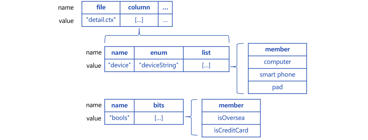
A special field definition is added under column. In the definition, name value is real field name bools in the physical table, and attribute bits contains a set of pseudo field names – there can be 16 boolean field names at most. Here bits value includes two field names, which correspond to the first bit and the second bit in the bools field value.

The SPL code for defining pseudo table p_detail is changed accordingly:

	A	B
1	=[{file:“detail.ctx”, column:[ {name:“device”,enum:“deviceString”,list:[“computer”,“smart phone”,“pad”]}, {name:“bools”,bits:[“isOversea”,“isCreditCard”]} ] }]
2	>p_detail=pseudo(A1)

A1 adds a special field bools. Attribute bits defines two pseudo field names.

Now part of data retrieved from pseudo table p_detail is as follows:

In subsequent computation, we directly use isOversea and isCreditCard to perform conditional filtering and grouping operation and display boolean values in the result set:

	A
	…
3	=p_detail.select(isOversea && (deviceString==“pad” || deviceString==“smart phone”))
4	=A3.groups(month@y(ddate):dmonth,deviceString,isCreditCard;sum(amt),count(~))

In A3, isOversea in the filtering condition will be automatically converted into the first bit of the bools value to filter physical table detail.

In A4’s result set, value of the second bit of bools field will be transformed to boolean value isCreditCard:

Appending data to a pseudo table only requires bit-based dimension pseudo field values. SPL will automatically convert them to real field values.

To append data to p_detail, for instance, it is enough that the new.btx to which data will be appended has isOversea,isCreditCard values. SPL will automatically convert them and generate real field bools. Following is the code:

	A
1	=[{file:“detail.ctx”, column:[ {name:“device”,enum:“deviceString”,list:[“computer”,“smart phone”,“pad”]}, {name:“bools”,bits:[“isOversea”,“isCreditCard”]} ] }]
2	>p_detail=pseudo(A1)
3	=file(“new.btx”).cursor@b(id,ddate,deviceString,amt,isOversea,isCreditCard)
4	=p_edtail.append(A3)

Suppose we update p_detail table according to the primary key and data of modify.btx and delete the table according to delete.btx’s primary key, the code is as follows:

	A
1	=[{file:“detail.ctx”, column:[ {name:“device”,enum:“deviceString”,list:[“computer”,“smart phone”,“pad”]}, {name:“bools”,bits:[“isOversea”,“isCreditCard”]} ] }]
2	>p_detail=pseudo(A1)
3	=file(“modify.btx”).import@b(id,isOversea,isCreditCard)
4	=file(“delete.btx”).import@b(id)
5	=p_edtail.update(A3:A4)

Redundant field

Suppose we add a record type custInfo field to physical table detail to store customer information in the transaction. This field has an attribute field comment, as shown below:

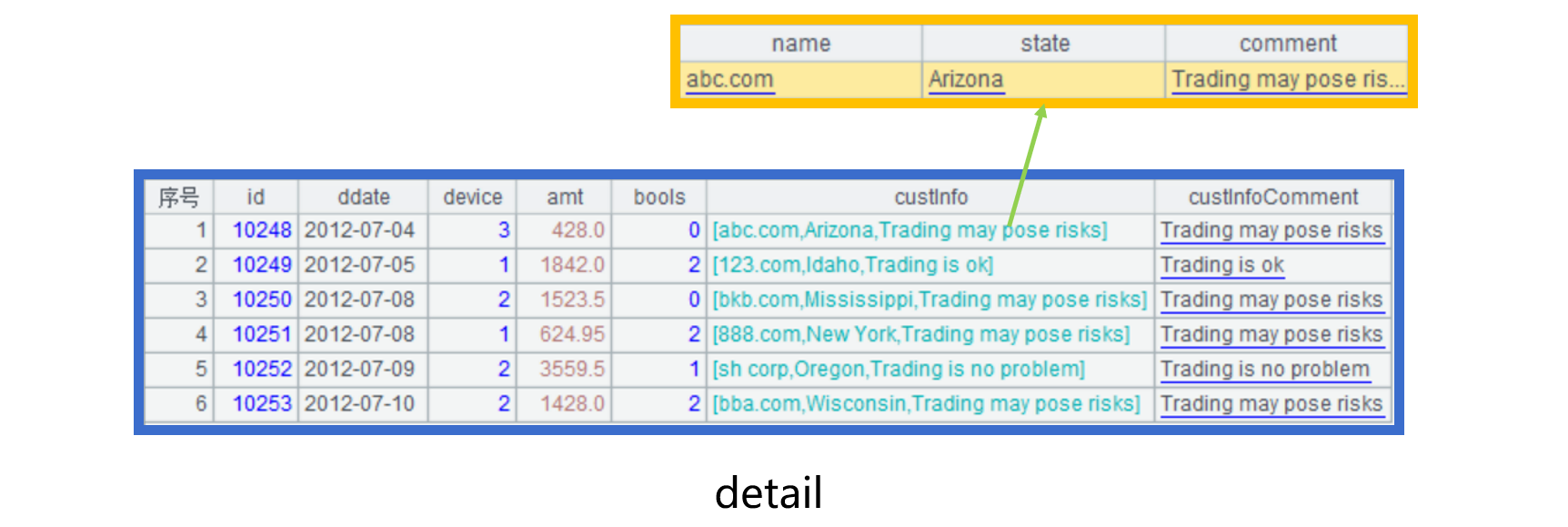
We need to perform a filtering to get data containing substring “risk” in each custInfo.comment string.

If we directly use custInfo.comment to peform the filtering, the whole custInfo field will be retrieved. Even if the other fields are not involved in the computation, they will still be read and parsed to form a whole record.

To increase performance, we can add a redundant field custInfoComment in the physical table to store custInfo.comment values. This helps reduce the amount of data to be read and get rid of the record generation process.

However, it is inconvenient because we need to specifically describe the relationship between the redundant field and the record type field. Yet even the description cannot make sure that programmers can make use of the redundant field in all suitable scenarios.

To tackle this problem, pseudo tables provide redundant field mechanism, which defines an expression exp for the redundant field. exp will be automatically replaced with the corresponding redundant field if it is involved in a relative computing expression:

In the above picture, we define the exp as custInfo.comment, and SPL automatically replaces custInfo.comment in a computing expression with custInfoComment field.

Now the pseudo table definition becomes this:

Below is the code of defining and using a redundant field:

	A	B
1	=[{file:“detail.ctx”, column:[ {name:“device”,enum:“deviceString”,list:[“computer”,“smart phone”,“pad”]}, {name:“bools”,bits:[“isOversea”,“isCreditCard”]} {name:“custInfoComment”,exp:“custInfo.comment”} ] }]
2	>p_detail=pseudo(A1)
3	=p_detail.select(pos(custInfo.comment,“risk”) && …)

A1: Define expression exp:“custInfo.comment” and the corresponding real field custInfoComment in the pseudo table definition.

A3: The filter condition contains the defined expression. Yet SPL will not retrieve records under custInfo and then their fields. Instead, the expression is directly replaced with the real field custInfoComment and participates in the subsequent computation using the redundant field value.

Appending data to and modifying data in a pseudo table just requires record field values. SPL will automatically convert them into the redundant field values. To append data to p_detail, for instance, the new.btx to which data will be appended just needs to contain custInfo and SPL will automatically convert it and generate custInfoComment. Below is the SPL code:

	A
1	=[{file:“detail.ctx”, column:[ {name:“device”,enum:“deviceString”,list:[“computer”,“smart phone”,“pad”]}, {name:“bools”,bits:[“isOversea”,“isCreditCard”]}, {name:“custInfoComment”,exp:“custInfo.comment”} ] }]
2	>p_detail=pseudo(A1)
3	=file(“new.btx”).cursor@b(id,ddate,deviceString,amt,isOversea,isCreditCard,custInfo)
4	=p_edtail.append(A3)

Suppose we update p_detail table according to the primary key and data of modify.btx and delete the table according to delete.btx’s primary key, the code is as follows:

	A
1	=[{file:“detail.ctx”, column:[ {name:“device”,enum:“deviceString”,list:[“computer”,“smart phone”,“pad”]}, {name:“bools”,bits:[“isOversea”,“isCreditCard”]}, {name:“custInfoComment”,exp:“custInfo.comment”} ] }]
2	>p_detail=pseudo(A1)
3	=file(“modify.btx”).import@b(id,custInfo)
4	=file(“delete.btx”).import@b(id)
5	=p_edtail.update(A3:A4)

Field aliases

In some applications, a real field has different meanings in different scenarios. We use pseudo table field aliases to represent their business meanings.

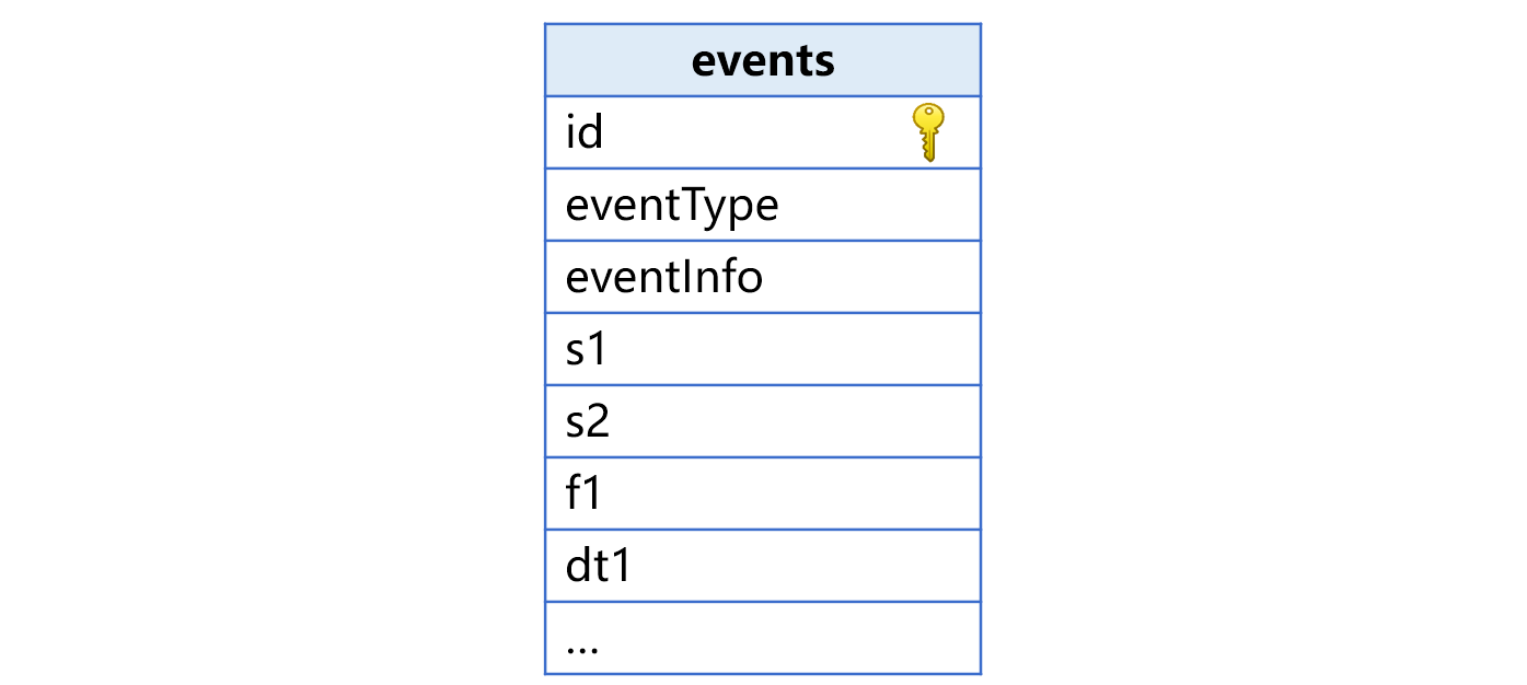
Take e-commerce system event table (events)as an example. In the table, each row corresponds to one event and each event stores event type (eventType) and property information of this type of event (eventInfo). eventInfo field is record type and contains multiple fields to store multiple properties.

Note that different types of events have different properties and same type of events have same properties. This means that eventType field value determines the number, names, and data types of fields under eventInfo record.

For instance, the relationship between eventType and properties of eventInfo is generally like this:

eventType	eventInfo
	property	data type
appInstall	browser	string
	device	string
	reward	float
appStart	page	string
	title	string
	dt	datetime
appEnd	page	string
	title	string
	amount	float
	dt	datetime
…	…

According to the above table, event type appInstall has three properties and appEnd corresponds to four completely different properties. Since there are a lot of event types and if we store each property as a field, there will be too many fields in the physical table. In fact, the number of properties each event type has is not too many.

One event can only correspond to one event type. Suppose an event is appInstall type and has a browser property, it is impossible that it has the page property under appStart type. Yet both are string, and we can use one real field s1 to store the two properties.

In this way, we can merge all properties of same data type in the following picture:

eventType	eventInfo		realField
	property	dataType
appInstall	browser	string	s1
	device	string	s2
	reward	float	f1
appStart	page	string	s1
	title	string	s2
	dt	datetime	dt1
appEnd	page	string	s1
	title	string	s2
	amount	float	f1
	dt	datetime	dt1
…	…	…	…

As the picture shows, real field s1 is used to store the three string type properties – browser, page and page under three event types. Besides, real fields s2, f1 and dt1 are defined to store properties of different data types respectively. In general, the four fields – s1, s2, f1 and dt1 are enough to store all properties listed above.

Now the physical table’s structure is as follows:

Though the number of fields in the physical table becomes much less, the field names do not imply any business meanings and are inconvenient to use. We need to interpret the field names according to eventType during the query, which makes coding more complicated.

To deal with this problem, we can use pseudo table’s field aliases and expression exp together. In the pseudo table, we specify multiple aliases having business meanings for each real field, as the following shows:

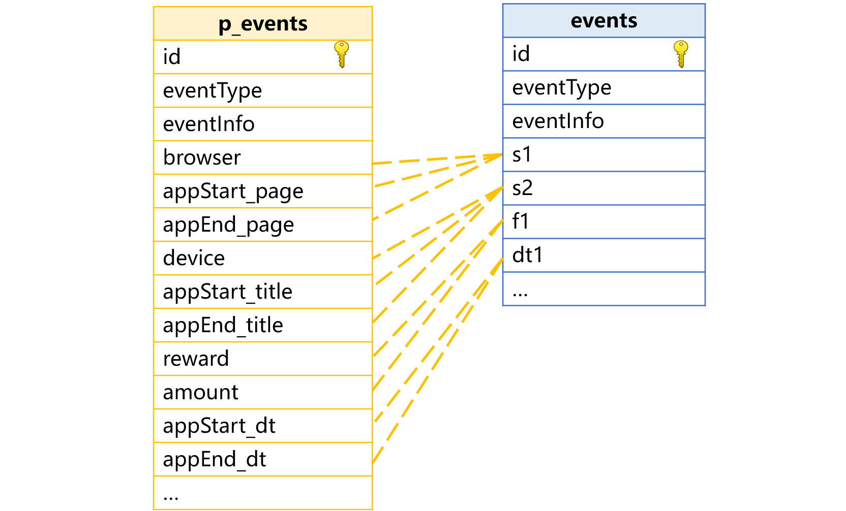
Aliases should not be duplicate, so certain aliases have event type prefix, such as appStart_page.

The eventType field in events table is defined as an enumerated dimension while stored as continuous natural numbers in the physical table.

Now the pseudo table definition becomes like this:

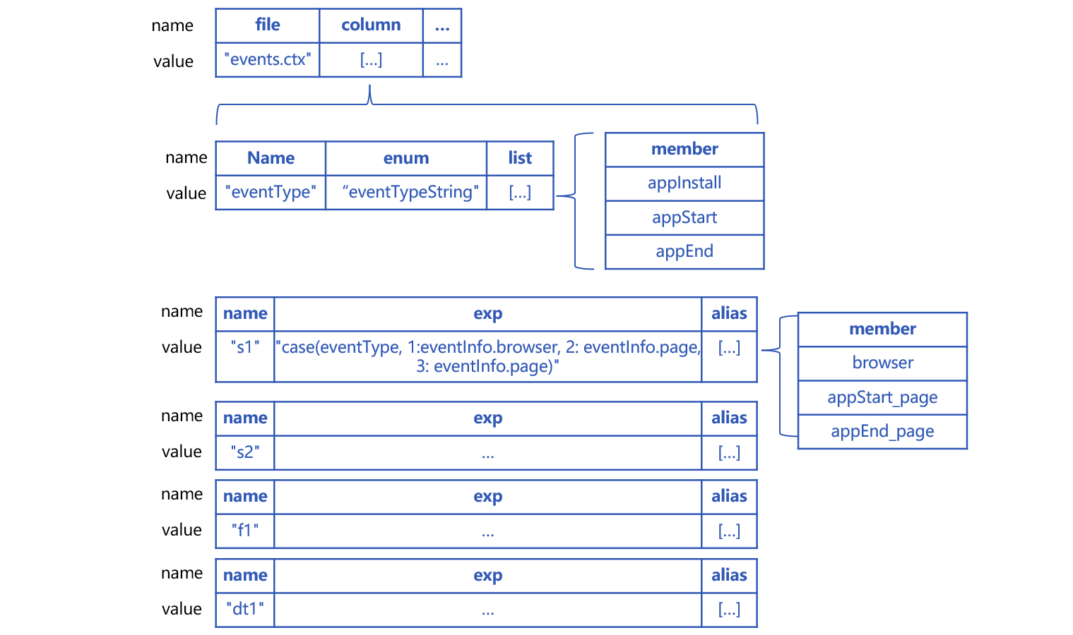
And the corresponding code is:

	A	B
1	=[{file:“events.ctx”, column:[ {name:“eventType”,enum:“eventTypeString”,list:[“appInstall”,“appStart”,“appEnd”]}, {name:“s1”,alias:[“browser”,“appStart_page”,“appEnd_page”],exp:“case(eventType, 1:eventInfo.browser, 2: eventInfo.page, 3: eventInfo.page)”}, {name:“s2”,alias:[“device”,“appStart_title”,“appEnd_title”],exp:“case(eventType, 1:eventInfo.device,2: eventInfo.title, 3:eventInfo.title)”}, {name:“f1”,alias:[“reward”,“amount”],exp:“case(eventType,1:eventInfo.reward,3: eventInfo.amount)”}, {name:“dt1”,alias:[“appStart_dt”,“appEnd_dt”],exp:“case(eventType,2:eventInfo.dt, 3: eventInfo.dt)”} ] }]
2	>p_events=pseudo(A1)
3	=p_events.select(eventTypeString==“appInstall” && browser==“firefox”)
4	=A3.import(id,eventTypeString,browser,reward)

A1: Define three aliases –“browser”,“appStart_page”,“appEnd_page” in the pseudo table for real field s1 and their corresponding expressions: exp:"case(eventType, 1:eventInfo.browser, 2: eventInfo.page, 3: eventInfo.page)".

If eventType value isn’t 1, 2 or 3, the value of real field s1 will be null. That’s why case(eventType, 1:eventInfo.browser;eventInfo.page) is incorrect.

Similar syntax for defining aliases for real fields s2, f1 and dt1.

A3: There is a field alias in the filter condition. SPL will not retrieve the records under eventInfo and then their fields. Instead, it automatically replaces it with the real field s1 and uses the redundant field value for subsequent computations.

A4: Retrieve the filter result.

Appending data to and modifying data in a pseudo table just requires event type field and record field values. SPL will automatically convert them into corresponding s1 and f1 fields, or other fields.

Suppose we append data to p_detail table, the new.btx file to which data will be appended only needs to have eventTypeString and eventInfo fields. SPL will automatically generate s1 field and f1 field according to the two fields. The code is as follows:

	A
1	=[{file:“events.ctx”, column:[ {name:“eventType”,enum:“eventTypeString”,list:[“appInstall”,“appStart”,“appEnd”]}, {name:“s1”,alias:[“browser”,“appStart_page”,“appEnd_page”],exp:“case(eventType, 1:eventInfo.browser, 2: eventInfo.page, 3: eventInfo.page)”}, {name:“s2”,alias:[“device”,“appStart_title”,“appEnd_title”],exp:“case(eventType, 1:eventInfo.device,2: eventInfo.title, 3:eventInfo.title)”}, {name:“f1”,alias:[“reward”,“amount”],exp:“case(eventType,1:eventInfo.reward,3: eventInfo.amount)”}, {name:“dt1”,alias:[“appStart_dt”,“appEnd_dt”],exp:“case(eventType,2:eventInfo.dt, 3: eventInfo.dt)”} ] }]
2	>p_events=pseudo(A1)
3	=file(“new.btx”).cursor@b(id,eventTypeString,eventInfo)
4	=p_events.append(A3)

Suppose we update p_detail table according to the primary key and data (id、eventTypeString、eventInfo) of modify.btx and delete the table according to delete.btx’s primary key, the code is as follows:

	A
1	=[{file:“events.ctx”, column:[ {name:“eventType”,enum:“eventTypeString”,list:[“appInstall”,“appStart”,“appEnd”]}, {name:“s1”,alias:[“browser”,“appStart_page”,“appEnd_page”],exp:“case(eventType, 1:eventInfo.browser, 2: eventInfo.page, 3: eventInfo.page)”}, {name:“s2”,alias:[“device”,“appStart_title”,“appEnd_title”],exp:“case(eventType, 1:eventInfo.device,2: eventInfo.title, 3:eventInfo.title)”}, {name:“f1”,alias:[“reward”,“amount”],exp:“case(eventType,1:eventInfo.reward,3: eventInfo.amount)”}, {name:“dt1”,alias:[“appStart_dt”,“appEnd_dt”],exp:“case(eventType,2:eventInfo.dt, 3: eventInfo.dt)”} ] }]
2	>p_events=pseudo(A1)
3	=file(“modify.btx”).import@b(id,eventType,eventsInfo)
4	=file(“delete.btx”).import@b(id)
5	=p_edtail.update(A3:A4)

Review & summary

A SPL pseudo table amounts to metadata, which makes the complex storage mechanisms used in physical tables transparent, and can be used as a simple table, reducing complexity of computations. In addition, pseudo tables can automatically map logically simple computations as high-efficiency computations based on the high-performance storage mechanism. This ensures the best computing performance possible.

After defining the enumerated field, bit-based dimension, redundant field, and field aliases in a pseudo table, we do not need to take care of storage mechanisms and computing methods and just treat it as a simple, common table.

Besides, pseudo tables can be used in user analysis scenarios to order data by two dimensions at the same time (Find details in SPL Pseudo Table Bi-dimension Ordering Mechanism ).