There is a phenomenon that in BI systems of some big organizations there are a lot of snapshot tables in their data warehouses. Take the BI system of a certain transaction business as an example. There are the huge transaction details table stored as a number of segment tables by month, and some tables that are not very large. The smaller tables, such as customer table, employee table and product table, need to associate with the larger transaction details table. At the end of each month, all data of these smaller tables are stored as snapshot tables in order to match the current month’s transaction details segment tables.

Why they need so many seemingly redundant snapshot tables?

The transaction details table is a familiar type of fact table. A fact table stores data of actual occurrences. And it will become larger as time goes by. There are various other kinds of fact table, such as orders table, insurance policy table and bank transaction records table. A fact table is often associated with other tables through certain code fields. For instance, transaction details table relates to customer table, employee table and product table through customer id, employee id and product id respectively, orders table relates to product table through product id field, and bank transaction records tables relates to user table through user id. These tables related to the fact table are called dimension tables. In the following figure, the transaction details table and the customer table have a relationship of fact table and dimension table:

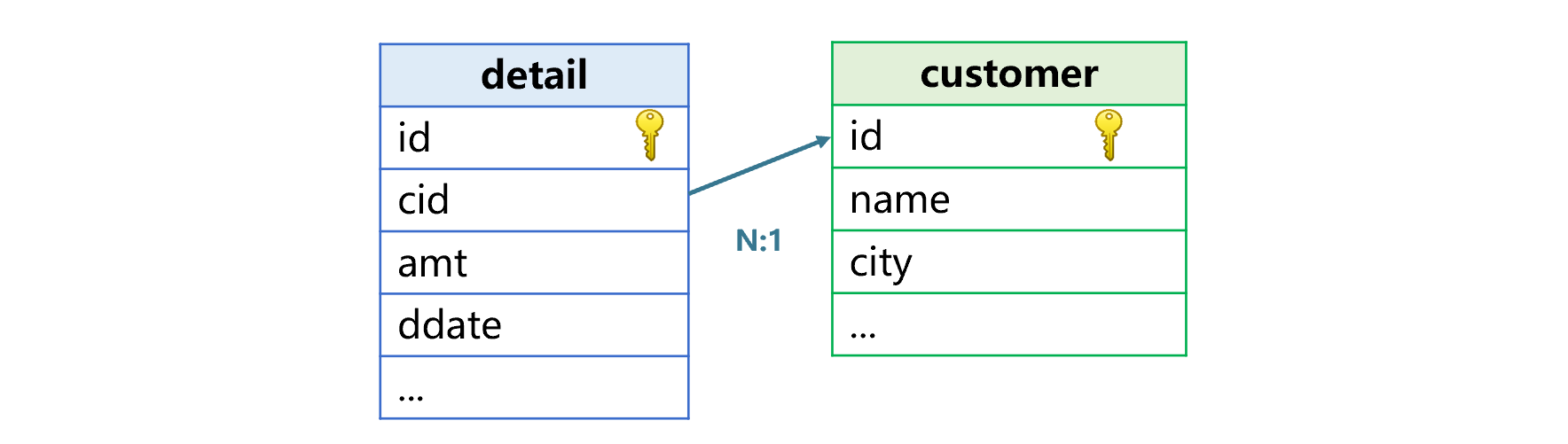
The reason of associating a fact table with a dimension table is that we need fields in a dimension table in computations. As the above shows, after joining detail table and customer table, we can group the former by customer’s city and calculate the total amount and count transactions in each group, or perform other computations.

Data in a dimension table is relatively stable though there are modifications. Update of a dimension table won’t affect the newly-generated data in the fact table, but it is likely that the fact table’s historical data does not match the dimension table’s new data. In this case, if we try to associate old data in the fact table with the new data in the dimension table, errors will occur.

Let’s look at an instance. There is a customer James whose code is B20101. He lived in New York and had some transaction records. He then moved to Chicago on May 15, 2020 and had new transaction details records. If we just change James’ city to Chicago in customer table, his transactions occurred in New York will be treated as in Chicago when we group detail records by customer’s city and calculate total amount in each city. That’s an error. The error occurs because which city a James’ transaction record belongs to is determined by time. Putting all records to either New York or Chicago is incorrect.

If we ignore the error, aggregate values on the historical data in the BI system and those on the newly-generated data in the ERP system will not match. And the mismatch errors are hard to detect.

Snapshot tables appear as a solution. Generate snapshot of a data table at a fixed time (such as at the end of each month), and store data of the fact table within a specified time period (like one month) and the whole data of the dimension table at that time for later analysis and computation. This way the fact table will be always related to the dimension table in the corresponding time, and aggregate values will be correct.

But this results in many redundant dimension data and increases database storage load. Moreover, there are multiple dimension tables, and each dimension table corresponds to multiple snapshot tables, causing extremely complicated inter-table relationships and greatly complexing the whole system.

Another consequence is that code becomes complicated. For example, there will be one transaction details table and a batch of dimension table snapshots for each month. If we want to group details records by customer’s city and calculate transaction amount and count transactions in each city within one year, we need to associate every month’s transaction details table with their dimension table snapshots and perform eleven UNIONs. This is just a simple grouping and aggregation operation. For more complicated analysis and computations, we will have very long and complex SQL statements. They are hard to maintain and even difficult to optimize. That’s why many BI systems that use the snapshot solution prohibit analysis and computations on data within a long time period. Sometimes they only allow computations on data in one unit time period (like one month).

The snapshot solution also cannot completely resolve the issue of incorrect query result resulted by the change of data in dimension tables. It is impossible for a BI system to generate a snapshot instantly each time when data in a dimension table is changed (if so, there will be too many snapshot tables and storage load will be huge). Generally, snapshot tables are only generated at specified time interval. Between the two time points when snapshot tables are generated, computing errors will still occur if there are any changes in dimension table data. Suppose snapshot tables for transaction details table and customer table are generated on the last day of each month and James moves from New York to Chicago on May 15, then on May 31 when the snapshot tables are generated, James’ city will be regarded and saved as Chicago. In June when we try to perform a query on data of May, errors will appear because James’ transactions from May 1 to 15 that should have been put under New York are mistaken for Chicago’s, though the error is not a serious one.

A workaround is to generate a wide table based on the fact table and the dimension table. According to this method, we join the transaction details table and the customer table to create a wide transaction table. In this wide table, information such as customer names and cities are not affected by the change of data in the customer dimension table. And this method ensures a simple data structure in the system. Yet, the same problem still exists. As the wide table is generated at a specified time interval (generating wide table records in real-time will be a drag on performance), any change of data in the dimension table between two generation time points will result in an error. What’s more, as the fact table and a dimension table have a many to one relationship, there will be a lot of redundant customer data in the wide transaction table, which leads to inflation of the fact table whose space usage will be far heavier than that of the snapshot tables. There’s one more problem. The wide table structure makes maintenance inconvenient, particularly when more fields need to be added, because we need to take care of the handling of the large volume of historical data. To make this simple, we have to specify as complete fields as possible when defining the wide table. A large and comprehensible wide table occupies larger space.

Let’s look at the issue in another way. Though dimension table data may change, it changes little. The amount of data updated is one or several orders of magnitudes smaller than the total data amount. Knowing this helps us use it to design a cost-effective solution.

The open-source data computing engine SPL uses this characteristic to design the time key mechanism. The mechanism can efficiently and precisely solve the issue caused by dimension table update.

The mechanism works like this. We add a time field in the dimension table. This new time field, which we call time key, and the original primary key field combine to form a new composite primary key. When joining the fact table and the dimension table, we create an association between the combination of the original foreign key field and a relevant time field in the fact table and the new composite primary key in the dimension table. This time-key-style association is different from the familiar foreign-key-style association. Records are not compared according to equivalence relations but are matched based on “the latest record before the specified time”.

Take the above transaction details table and customer table as examples. We add an effective date field edate to the customer table, as the following figure shows:

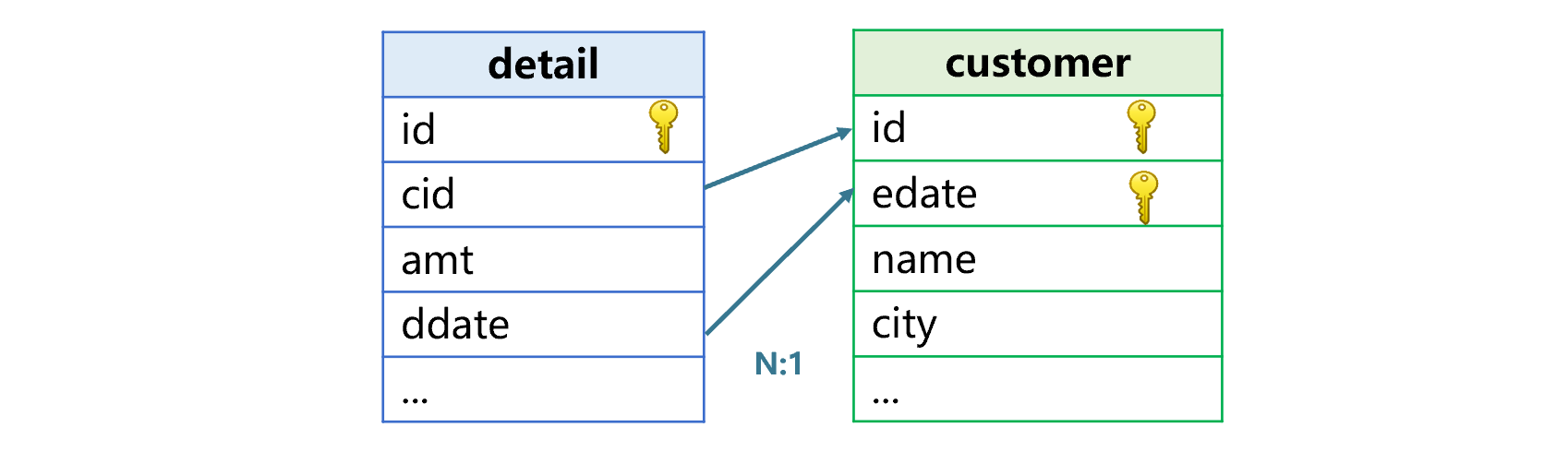
edate field contains the date when the current record appears, that is, the date when an update occurs. For instance, below is the customer table after James moves to Chicago:

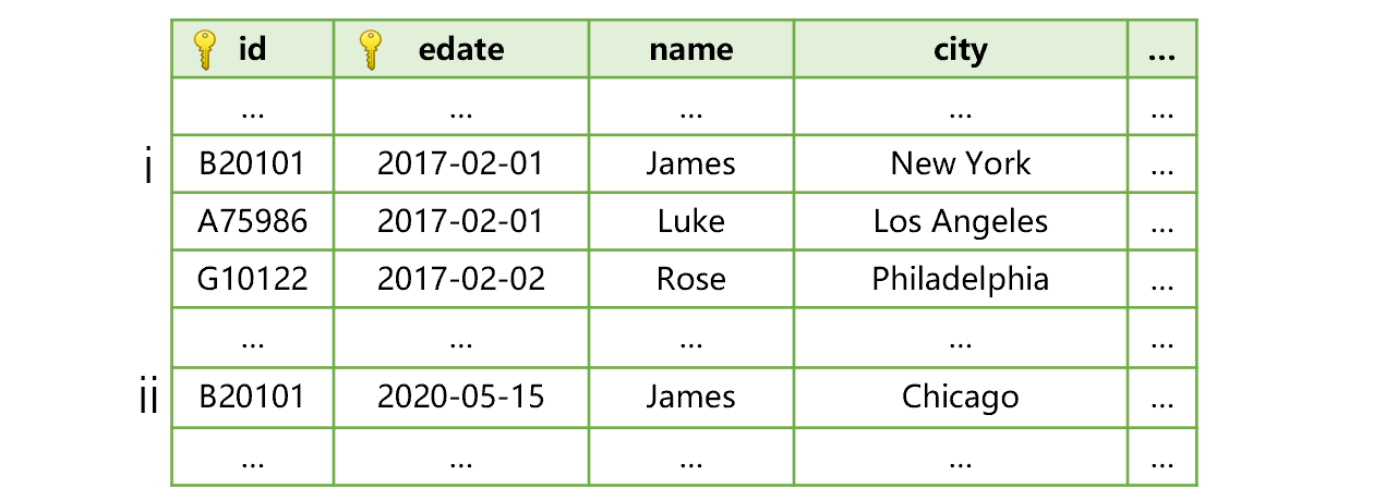
As above shows, James has only one dimension record i before he moves to Chicago, and on the date when he moves record ii appears. The effective date is the date when he moves, which is 2020-05-15.

In this case, the SPL join between transaction details table and customer table will, except for comparing values between cid and id, also compare values between ddate and edate that records the record’s time of appearance and find out the record having the largest edate value that is not greater than ddate. This is the correct matching record (which is the latest record before the specified time point). As transaction records before James’ relocation are all before 2020-05-15, they will relate to record i in customer table where the effective date is 2017-02-01 and will be regarded as belonging to New York. The transaction records after James’ relocation fall on or after 2020-05-15, so they will relate to record ii where the effective date is 2020-05-15 and put under Chicago.

By using the time key mechanism, the joining result conforms to the facts. SPL can obtain correct results in later computations because it adds a record to the dimension table and stores the effective date at the time when the update occurs. The approach avoids the problem caused by generating snapshots and wide tables at regular time, and thereby getting rid of errors in performing computations within two regular time points.

Changes of data in a dimension table are small. There is little change in the size of a dimension table after the effective time information is added. Storage load will not increase noticeably.

In theory, we can add similar time field in a dimension table in the relational database. The problem is that we cannot express the join relationship. Obviously, the time-key-based association is not the commonly seen equi-join. Even if we try to use the non-equi-join to achieve the association, we need the complex subqueries to select the latest dimension table records before we perform the join. The statement is too complicated and the performance is unstable. With relational databases, we have no choice but using the snapshot/wide table solution.

The SPL code for achieving the time key mechanism is simple, as shown below:

A1 imports the customer table. B1 defines a new composite primary key using id and edate; @t option means the last field of the primary key is a time key. We can use the high-precision datetime field as the time key as needed.

A2 creates cursor for the transaction details table.

B2 creates association between A2’s cursor and A1’s customer table. The detail table’s joining fields are cid and ddate, and the customer table’s is the primary key. The operation works the same as one between regular dimension tables without a time keys.

A3 groups records in the joining result set by customer’s city, and calculates total amount and counts transactions in each city. In this step time keys are not involved.

The time key mechanism is one of SPL’s built-in features. The performance gap between a computation using the mechanism and one without using it is very small. Same as joins involving regular dimension tables, one can perform aggregations on any time ranges. There are no time limits as snapshot approach has.

The SPL time key mechanism deals with dimension data change issues in a convenient way. The fact table remains what it is, and we add a time field to the dimension table and record data change information only. The design ensures correct result and good performance while eliminating a large number of snapshot tables and reducing system complexity. It also avoids serious data redundancy resulted from wide table solution, and maintains a flexible system architecture.