

Comparison between SPL and Python in processing structured data
Overview
SPL is designed primarily to address the difficulties of SQL (difficult to code and slow to run for complex task, difficult to perform cross-source calculation, dependent on stored procedure), and its application scenarios are similar to those of SQL. SPL generally works with application, and supports big data, including high-performance operation and parallel computing. Likewise, Python can help solve SQL’s problem that is difficult to code when facing complex task. However, Python is developed from desktop programming language, and has little ability to work with application and weak ability in big data and parallel computing. Nevertheless, since Python is incredibly popular in the AI world, boasting a wealth of third-party libraries and algorithms such as Sklearn, TensorFlow and PyTorch, it seems that Python has become the number one language in AI. In contrast, SPL is relatively weak in AI and only provides part of functions. Both SPL and Python can be used to simplify the cumbersome syntax of structured data operation, but we will find that they are still quite different when we look deeper. In short, SPL is deeper in understanding the structured data, more complete in computing ability, and better in syntax consistency.Understanding of structured data
Data table
SPL not only inherits the concepts of table and record in SQL (record is an object with attributes (field), and table is a set of records of the same structure), but extends SQL, allowing records to be independent from table, and allowing records from different tables to form new set to participate in operations. In contrast, Python does not have explicit concept of table or record. In Python, the DataFrame, which is often used to represent structured data, is essentially a matrix with row and column indexes, and the column index is usually a string that can be regarded as field name. Structured data is often presented as the form of a two-dimensional table, which also looks like a matrix at a glance. For simple basic operation, it indeed works almost the same way, but for slightly complex operation, differences in understanding occur, resulting in the inability to code in a natural way. Let's take a simple filtering operation as an example. Here below is an employee data table: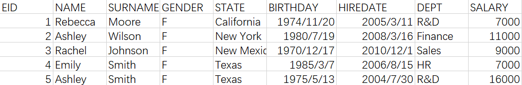
import pandas as pd
data = pd.read_csv('Employees.csv')
#Filtering
rd = data.loc[data['DEPT']=='R&D']
print(rd)
As we can see that this code is very simple, and the result is correct, but, the used function is called loc (the abbreviation of location), which has nothing to do with filtering. In fact, the filtering in this code is implemented by locating the row index that satisfies the condition. The data[‘DEPT’]==’R&D’ in the function will calculate a boolean value Series (as shown in the figure below, the index is the same as that of data, and the row that satisfies the condition is set as True, otherwise False), and then loc fetches the data by the row index of True, which is a matrix operation in essence.
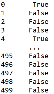
Boolean Series
In addition, DataFrame can be filtered not only with locfunction, but also with other methods like query(…).Essentially, however, it is to locate the row or column index of matrix, and then fetch the data by row or column index, writing as matrix.loc[row,col] in general.
By contrast, SPL is to filter out records that meet the condition from the data table directly.
A |
B |
|
1 |
=file(”Employees.csv”).import@tc() |
Read data/ |
2 |
=A1.select(DEPT==”R&D”) |
Filter out subset/ |
This code is in line with the thinking of set operation.
Let's attempt to do a simple operation on the filtered subset. For example, modify the data in the subset.
Task 2: Raise the salaries of employees of R&D department by 5%:
According to natural thinking, we just need to filter out the employees of R&D department and then modify their salaries.
Python code based on this logic:
import pandas as pd
#Read data
data = pd.read_csv('Employees.csv')
#Filter out employees of R&D department
rd = data.loc[data['DEPT']=='R&D']
#Modify salaries
rd['SALARY']=rd['SALARY']*1.05
print(data)
Not only does this code trigger a run warning, but it also does not modify SALARY.
This is because rd = data.loc[data[‘DEPT’]==‘R&D’] is a filtered matrix, and when modifying SALARY on it, it actually modifies the submatrix rd, but the original matrix data.
Then, how to code correctly?
import pandas as pd
data = pd.read_csv('Employees.csv')
#Find the salaries of employees of R&D department
rd_salary = data.loc[data['DEPT']=='R&D','SALARY']
#Clip out the salaries of employees of R&D department and modify
data.loc[data['DEPT']=='R&D','SALARY'] = rd_salary*1.05
print(data)
Python's subset is a new matrix, so if we want to modify the salaries of a department, we have to fetch them out first (corresponding statement in this code: rd_salary =...), and if we want to raise them by 5%, we have to do one more step, that is, clip out them from the original matrix, and then modify them with the fetched data. This coding method requires repetitive filtering, which is not only inefficient but too complicated.
Unlike Python, SPL regards a table as a set of records, and filtering is to take a subset, and the only thing we need to do next is to modify the data of subset according to normal thinking. SPL code:
A |
B |
|
1 |
=file(”Employees.csv”).import@tc() |
Read data/ |
2 |
=A1.select(DEPT==”R&D”) |
Filter out subset/ |
3 |
=A2.run(SALARY=SALARY*1.05) |
Modify the subset/ |
A2(employees of R&D department) is a subset of A1(employeetable). Since A2is just a reference of A1, the original set A1will be modified at the same time when A2is modified.
Operation
In addition to different understandings of data type, there are differences between SPL and Python in the understanding of operations, such as common aggregation operation.
Python, like SQL, specifies the aggregation operation result as a single value, such as sum, count, max and min. But SPL is different. In SPL, extracting any information from a large set is regarded as an aggregation operation. For example, select the member with max or min value.
When we want to see the information of member with maximum salary:
Coding in Python is like this:
import pandas as pd
#Read data
emp = pd.read_csv('Employees.csv')
#Select the member with maximum value (1 member)
#Index of the member with maximum salary
max_salary_idx=emp.SALARY.argmax()
#Member with maximum salary
max_salary_emp=emp.loc[max_salary_idx]
print(max_salary_emp)
#Select the members with maximum value (multiple members)
#Maximum salary
max_salary=emp["SALARY"].max()
#Select by maximum salary
max_salary_emp=emp[emp.SALARY==max_salary]
print(max_salary_emp)
Since Python does not regard “extracting the member where the maximum value is located” as an aggregation function, this task is done in two steps. The first step is to use argmax()to get the index of target value, and the second step is to select the member by index. Moreover, argmax()can only return the index containing only one member with maximum value. If we want to return all members with maximum value, we need to traverse the data twice (one is to calculate the maximum value, the other is to select the members), which is undoubtedly much more troublesome.
In contrast, SPL regards such operation as an operation that is not much different from sum, count, etc. All of these operations are regarded as aggregation operation, and they extract the information from large set. SPL code:
A |
B |
|
1 |
=file(”Employees.csv”).import@tc() |
|
2 |
=A1.maxp(SALARY) |
#1 member with max value |
3 |
=A1.maxp@a(SALARY) |
#All members with max value |
The aggregate function maxp() returns the member where the maximum value is located, and returns all target members when adding the option @a, which is not fundamentally different from conventional aggregate functions such as sumand count. Their usage is the same, but maxp() is simpler to code.
SPL also provides operation that returns the sequence number where the maximum value is located like argmax. Likewise, this operation is still regarded as an aggregate function.
A |
B |
|
1 |
=file(”Employees.csv”).import@tc() |
|
2 |
=A2.pmax(SALARY) |
/Location of 1 member with max value |
3 |
=A2.pmax@a(SALARY) |
/Location of all members with max value |
We can see that both the syntax and style are the same.
A similar operation is TOPN. Python doesn’t regard TOPN operation as aggregation operation, and will sort first, and then take the first N. SPL advocates universal set, and the result of aggregation operation may be a set. Similar to sumand maxp, calculation can be done directly in SPL without having to do sorting first.
There are also many operations that are understood differently between SPL and Python. For example, the join operation, Python continues to use SOL’s concept, defining the join as Cartesian product andthen filtering. Although it is widely applicable, it lacks some key features, resulting in failure to simplify coding and optimize the performance. SPL, on the other hand, categorizes the most common equijoin and requires primary keys to be associated, eliminating the many-to-many relationship, and making it possible to reference associated fields directly in the code under such definition to simplify coding, and it will not generate incorrect logic as a result of missing the association condition, and also optimize the operation performance by utilizing primary key.
In summary, Python's understanding of data table and operation is not as deep as that of SPL, resulting in a difficulty of implementing the operation according to natural thinking. For basic operations, the difficulty is not obvious, but for slightly complex operations, it will be more difficult to code.
Completeness of operations
SPL is also designed richer than Python in structured data operation, let’s take the ordered computing, which SQL is not good at, to illustrate.
The set in SPL is ordered, allowing us to reference set member by sequence number. The DataFrame in Python is ordered as well, and the member can also be accessed by sequence number (row index). Both Python and SPL support the most basic ordered operations, which is what SQL lacks, resulting in a difficulty of coding in SQL for ordered operation, this is one of the reasons why SPL and Python can solve the difficulty of SQL.
However, for complex and in-depth scenarios, the gap between SPL and Python widens.
Adjacent reference
Adjacent reference is a common ordered operation. For example, calculating the daily rising/falling rate of a stock needs to reference the previous row of data when traversing. Since Python doesn’t provide the functionality of getting adjacent data, it needs to use a method of shifting the matrix index first, and then calculating the rising/falling rate with the shifted data and original data. Python code is like this:import pandas as pd
#Read data
stock_62=pd.read_csv(“000062.csv”)
#Shift by 1 row
stock_62s=stock_62["CLOSING"].shift(1)
#Calculate the rising/falling rate
stock_62["RATE"]=stock_62["CLOSING"]/stock_62s-1
print(stock_62)
SPL provides the symbol []to get adjacent data, and its code is very concise.
A |
B |
|
1 |
=file(“000062.csv”).import@tc() |
/Read data |
2 |
=A1.derive(if(#==1,null,CLOSING/CLOSING[-1]-1):RATE) |
Add rising/falling rate/ |
Ordered grouping
Grouping in SQL only cares about grouping key value, and doesn’t care about data’s order. However, some grouping operations are related to order, such as the operation whose grouping condition involves adjacent members, which is a headache for SQL. For example, there is a string consisting of letters and numbers “abc1234wxyz56mn098pqrst”, and we want to split it into smaller strings “abc,1234,wxyz,56,mn,098,pqrst”. Like SQL, grouping in Python only cares about key value, so we have to rack our brains and adopt an indirect way to implement key-value grouping by creating a derived column. Python code:import pandas as pd
s = "abc1234wxyz56mn098pqrst"
#Create Series
ss = pd.Series(list(s))
#Judge whether it is a number
st = ss.apply(lambda x:x.isdigit())
#Derive a Series that judges whether adjacent data are equal
sq=(st != st.shift()).cumsum()
#Group by derived column
ns =ss.groupby(sq).apply(lambda x:"".join(x))
print(ns)
SPL provides the option @ofor grouping, allowing us to put the same data adjacent to each other into one group and create a new group when data changes.
A |
B |
|
1 |
abc1234wxyz56mn098pqrst |
|
2 |
=A1.split().group@o(isdigit(~)).(~.concat()) |
Create a new group when value changes/ |
Positioning calculation
Positioning calculation refers to an operation whose logic is related to the involved data and the position of the set in which the data is located, which is also a common operation in data analysis. For example, when we want to calculate the rise of a stock in three days when its prices are maximum, not only do we need to use the stock prices (data itself) of the three days (members), but we also need to use the stock price of the day before the three days (operation on data location). Calculate the rise of a stock in three days when its prices are maximum. Since Python is unable to compute against the position information of data during the loop, it has to adopt an indirect way, that is, first find the index of the three days when its prices are maximum, and then shift the data, and finally calculate the rise based on three maximum prices and shifted data. Python code:import pandas as pd
#Get the information of stock (000062)
stock_62=pd.read_csv(“000062.csv”)
#Position after sorting
sort_pos=(-stock_62["CLOSING"]).argsort()
#Positions of 3 days when stock prices are maximum
max3pos=sort_pos.iloc[:3]
#Shift the data
stock_62s=stock_62.shift(1)
#Information of stock price of 3 days when stock prices are maximum
max3CL=stock_62["CLOSING"].iloc[max3pos]
#Information of stock price of the day before the 3 days when stock prices are maximum
max3CLs=stock_62s["CLOSING"].iloc[max3pos]
#Calculate the rising/falling rate
max3_rate=max3CL/max3CLs-1
print(max3_rate)
SPL provides the calcfunction, which uses the symbol []to get adjacent data, and uses the position and relative position of the members to perform calculation.
A |
B |
|
1 |
=file(“000062.csv”).import@tc() |
|
2 |
=A1.psort@z(CLOSING) |
/Positions of sorted stock prices |
3 |
=A2.m(:3) |
/Select the first 3 positions |
4 |
=A1.calc(A3,if(#==1,null,CLOSING/CLOSING[-1]-1)) |
Calculate the rising rate by position/ |
We can also use theptop(...)functionto calculate the position information of the three highest stock prices. Likewise, this function can return same position information, which is the TOPNoperation mentioned above. The difference is that the topreturns the members, while the ptopreturns the member positions, both of them belong to aggregation operation. In this way, A2is no longer needed, A3=A1.ptop(-3,CLOSING), and A4remains unchanged.
Non-equivalence grouping
In addition to ordered operation, SPL provides many operations that are designed more complete than Python, such as non-equivalence grouping. The original intent of the grouping operation is to divide a large set into several subsets according to a certain criterion. SPL exactly follows this natural thinking, that is, it provides both equivalence grouping (complete partition) and non-equivalence grouping (incomplete partition). In contrast, Python only provides equivalence grouping, and has to adopt an indirect way to implement non-equivalence grouping. Let's look at an example of non-equivalence grouping: Count the number of male employees in the specified departments ['Administration', 'HR', 'Marketing', 'Sales'] of a company. Because there may be other department except the four departments listed above (this may result in a situation where some members are not assigned to any group), or there may be department that does not have male employee (resulting in an empty subset), and Python can only perform equivalence grouping, it has to do one more step, that is, align with the help of function merge. Python code:import pandas as pd
#User-defined alignment grouping function
def align_group(g,l,by):
d=pd.DataFrame(l,columns=[by])
m=pd.merge(d,g,on=by,how='left')
return m.groupby(by,sort=False)
file="D:\data\EMPLOYEE.csv"
#Read data
emp=pd.read_csv(file)
#Select out male employees
emp_f=emp.query('GENDER=="M"')
sub_dept=['Administration','HR','Marketing','Sales']
#Alignment grouping
res=align_group(emp_f,sub_dept,'DEPT').EID.count()
print(res)
SPL, by contrast, is much smarter. SPL provides an alignment grouping function, we only need to align the groups by specified departments.
‘ |
A |
B |
1 |
D:\data\EMPLOYEE.csv |
|
2 |
=file(A1).import@tc() |
|
3 |
=A2.select(GENDER=="M") |
/Select male employees |
4 |
[Administration, HR, Marketing, Sales] |
/Specify departments |
5 |
=A3.align@a(A4,DEPT).new(A4(#):DEPT,~.len():NUM) |
/Aggregate the aligned groups |
This example only introduces two characteristics of non-equivalence grouping (one is that there may be members who are not assigned to any group, and the other is that there may be a group that is empty subset). In addition, there is a situation where member is assigned to different groups, which is more difficult for Python, yet for SPL, it is simple, we only need to use the function enum@r(). For more information, please visit: Python vs. SPL 7 -- Alignment Grouping & Enumeration Grouping.
Python does not provide complete operations. Although the above tasks can be implemented using basic operations (shifting the index, grouping, getting position, etc.), the computing idea is complicated and the code complexity is high. In contrast, SPL provides relatively complete operations, and the computing idea is simple and straightforward, and it only needs one or two lines of code to implement key calculations.
Syntax consistency
As a programming language, there should be a systematic approach to solving similar problems. Only in this way can we draw inferences by analogy easily and bring this language into full play. Python doesn't do a good job in this regard. As mentioned earlier when introducing the aggregate function, the syntax of returning one member with maximum value is quite different from that of returning multiple members (this can also be explained as the completeness problem caused by different operation understandings). Let's look at some more direct examples. In the adjacent reference discussed above, Python uses the function shift() to implement calculation, and now let's look at a similar problem: Calculate the moving average of a stock in 5 consecutive trading days. This problem is similar to the previous problem that calculates the rising/falling rate of the day, both are to obtain adjacent data to implement calculation, the only difference is to obtain one row or multiple rows of data. Python code:import pandas as pd
#Read data
stock_62=pd.read_csv(“000062.csv”)
#Shift by 1 row
stock_62["MAVG"]=stock_62["CLOSING"].rolling(5,min_periods=1).mean()
print(stock_62)
Although Python can't get adjacent members, it should continue to utilize the function shift()that is used in previous task, but it doesn’t. Instead, it uses a new function rolling(), this way of handling is like “one problem, one solution”, which is puzzling.
It is much simpler in SPL. SPL continues to use the symbol [], the only difference is that it was to take the data of 1 adjacent row, and now it is to take the data of 4 adjacent rows.
A |
B |
|
1 |
=file(“000062.csv”).import@tc() |
/Read data |
2 |
=A2.derive(CLOSING[-4:0].avg():DAY5) |
Moving average/ |
A similar problem is the function in positioning calculation mentioned above. This function is to obtain the member position after sorting. In that case, the function argsort()was used since there was only one sorting key. However, when multiple columns of keys are sorted by different order to obtain the position information, argsort()does not work, we need to use another function lexsort().
Calculate the position/index after sorting by the stock code in ascending order and stock price in descending order.
Python code:
import pandas as pd
stock_file="D:/data/STOCKS.csv"
#Read data
stock_data=pd.read_csv(stock_file,dtype={'STOCKID':'object'})
import numpy as np
#Get position information
sort2key_pos=np.lexsort((-stock_data["CLOSING"],stock_data["STOCKID"]))
print(sort2key_pos)
Python's lexsort()function is not in pandas but in numpylibrary. In addition, this function cannot sort in reverse order, it has to represent the reverse order with a minus sign “-”. However, Python doesn’t support the minus sign in strings. Therefore, the functionlexsort() will not work if the calculation is to sort by STOCKIDin descending order and by CLOSINGin ascending order, we have to find another method.
In SPL, the whole calculation is much easier, and we just continue to use the function psort().
SPL code:
A |
B |
|
1 |
D:\data\STOCKS.csv |
|
2 |
=file(A1).import@tc(#1:string,#2,#3) |
/Read data |
3 |
=A2.psort(STOCKID,-CLOSING) |
/Sorted positions/indexes of multiple columns in different directions |
Whether it's a single column or multiple columns, sorts in ascending order or descending order, the function psort() works, and SPL supports the minus sign in strings (-STOCKIDis to sort in reverse order).
In terms of data structure, both the native Python and the third-party libraries design different data structures. Take the set as an example, Python has various forms of structures including the list, set, array, Series andDataFrame, and each data structure has its own use scenarios. Although these structures can be converted to each other, the inconsistency of syntax rules brings a lot of troubles to users. In contrast, SPL does much better. To be specific, SPL has only two types of sets, sequence and table sequence. Technically speaking, SPL has only one type of set, i.e., the sequence (or ordered set), as the table sequence is a sequence composed of records. When calculating, as long as we master the calculation rules of sequence, we can draw inferences by analogy and solve similar problems with the same method.
In summary, Python is like a wildly growing plant. Although it has strong adaptability and can always find a way to solve a problem, it is too complicated sometimes, and it is not easy to draw inferences about other cases from one instance, so Pythonis not only computationally inefficient, but brings a bad user experience.
In contrast, SPL is an elaborately designed language with better syntax consistency, making it easier to draw inferences about other cases from one instance, and hence it has the ability to implement various computing tasks.
Lambda syntax
In terms of basic program logic, both Python and SPL provide complete function, such as branch flow, loop flow and subprogram, which is where they surpass SQL, and is another reason why they are suitable for solving the complex problems of SQL. Python and SPL are both the dynamic language, and have the concept of loop function. Both of them can use Lambda syntax to avoid writing cumbersome loop statement. For example, calculate the sum of squares of the first 100 integers. Python code:import pandas as pd
#1 to 100
l=[i for i in range(1,101)]
#Create Series
s=pd.Series(l)
#Sum of squares
odd_sum=s.apply(Lambdax:x*x).sum()
print(odd_sum)
Lambda syntax in Python is relatively conventional. When there is a loop, we need to set a parameter (x)to represent the current member first, and then execute the desired operation on the parameter (x).
In contrast, SPL does not define the parameter variable used in Lambda syntax, and instead uses a fixed symbol “~”, which is simple in coding, eliminating the need to define variable.
SPL code:
A |
B |
|
1 |
=to(100) |
/Generate a sequence |
2 |
=A1.sum(~*~) |
/Represent the current element with symbol ~ |
The fixed symbol undoubtedly makes coding simple, but it will cause trouble. For example, when there are nested loops, confusion occurs in the recognition of symbol ~. In this case, we have to define variables to distinguish the variable of every layer of loop.
For example, calculate the distance between every two numbers of the first 100 numbers.
A |
B |
|
1 |
=to(100) |
/Generate a sequence |
2 |
=A1.((v=~,A1.(abs(v-~)))) |
/Calculate the distance between every two numbers |
SPL specifies that the symbol ~only represents the members of the loop at innermost layer, and the members of outer-layer loops must be indicated by defining additional variables.
In the above example, the computing object of Python is Series, while that of SPL is a sequence. If there is a structured Dataframe or table sequence, what should we do?
We just need to organize the first 100 numbers as aDataframe, and name the field “value”. Python code:
import pandas as pd
#1 to 100
l=[i for i in range(1,101)]
#l1=[i for i in range(1,101)]
#Create Series
df=pd.DataFrame(l,columns=["value"])
#Sum of squares
odd_sum=df.apply(lambdax:x.value*x.value,axis=1).sum()
print(odd_sum)
As we can see from the code that the Lambda syntax of Python can work on Dataframe, but can't reference the field directly, it needs to use the symbol “.” to get the data, which is cumbersome for structured data operation involving many fields.
SPL, like SQL, can reference the field directly in Lambda syntax.
SPL code:
A |
B |
|
1 |
=100.new(~:value) |
/Generate a table sequence |
2 |
=A1.sum(value*value) |
/Calculate with field name |
From the above example alone, we can see that the difference between Python and SPL in Lambda syntax is just in form, not in essence. In fact, SPL's Lambda syntax is richer in that it can get not only the members of current loop, but the index of current loop members, and adjacent members.
For example, here below is a company’s monthly sales of one year:
[123,345,321,345,546,542,874,234,543,983,434,897]
Now we want to calculate the maximum monthly increase.
SPL represents the sequence number of current member with the symbol #, and specifies that the increase of the first month is 0, and gets the data of adjacent member with the symbol []. The following code is to calculate the increase of each subsequent month:
A |
B |
|
1 |
[123,345,321,345,546,542,874,234,543,983,434,897] |
/Monthly sales |
2 |
=A1.(if(#==1,0,~-~[-1])).max() |
/Maximum monthly increase |
Since the Lambda syntax of Python can't get the sequence number of current member and the data of adjacent members, it has to abandon Lambda syntax and adopts other ways instead.
Python code:
import pandas as pd
amt=[123,345,321,345,546,542,874,234,543,983,434,897]
s=pd.Series(amt)
ss=s.shift()
ma=(s-ss).fillna(0).max()
print(ma)
This task can also be written with the for loop of native Python, which is not troublesome. However, it is not Lambda syntax, so we won’t discuss it here.
We’ve already employed # and [] when comparing SPL and Python in adjacent reference section, the two symbols make Lambda syntax more convenient and SPL operation more complete.
The ability to process big data
Computing in external storage
Python’s ability to process big data is very weak, and hardly provides the method for big data operation. To implement some very simple big data calculation tasks, we have to hard-code ourselves. SPL, by contrast, has a complete cursor mechanism, which allows us to process big data easily. Moreover, most of the cursor functions are used almost the same way as memory functions and very user friendly.
Let's take the grouping and aggregating operation of big data as an example to explain the difference between SPL and Python.
We have the order data of a company (involving the order in each state of the U.S., and the amount of data is too large to be stored in memory of a single machine), now we want to aggregate the sales of each state.
Calculation idea: group the data by state, and aggregate the sales of each state.
SPL creates a cursor for order data, and then performs grouping and aggregating operation on the cursor. The code is written as follows:
A |
B |
|
1 |
D:\data\orders.txt |
|
2 |
=file(A1).cursor@t() |
/Create a cursor |
3 |
=A2.groups(state;sum(amount):amount) |
/Group and aggregate |
From the code in A3alone, we can't tell it is an in-memory calculation or a cursor calculation, because this statement is exactly the same as that used in in-memory calculation. However, the cursor calculation has something special. For example, if we want to group once more by another field (like the place of production), then we just write another groupsstatement in the case of in-memory calculation, but this method does not work in cursor calculation, because we cannot fetch the records due to the end of traversal. In this case, we need to re-create a new cursor and then write groups statement again.
To implement this grouping and aggregating task in Python, we need to read the data in segments first, and then group and aggregate the data of each segment, and finally group and aggregate the grouped and aggregated result of previous step. In addition, consideration should be given to the length of segment, otherwise it may result in a failure to read the data of segment into memory or the memory cannot hold the grouped and aggregated result. Does it sound annoying? Actually, it would be more annoying in coding. This is merely an example of aggregating after grouping, and does not need to code the grouping process. Sometimes, however, the grouping process needs to be coded in Python, which involves the hard coding of hash grouping. In that case, it is not easy even for advanced engineers due to high complexity of coding.
Parallel computing
The parallel computing in Python is just to simulate the method of parallel computing, but for CPU, it is actually the single-core running, so Python has no parallel computing ability in essence.
In contrast, SPL not only provides complete parallel computing ability, but supports the multipurpose traversal of cursor.
Again, let's take the order data just mentioned as an example. Now we want to count each state’s number of orders (order with sales greater than $500,000), while aggregating the sales of each state.
SPL code:
A |
B |
|
1 |
=file("D:\data\orders.txt").cursor@tm(area,amount;4) |
|
2 |
cursor A1 |
=A2.groups(state;sum(amount):amount) |
3 |
cursor |
=A3.select(amount>=50).groups(state;count(1):quantity) |
SPL offers @moption to create a parallel multi-cursor, and automatically computes in parallel and gets a correct result. Moreover, SPL implements the multipurpose traversal through channel, which not only makes full use of the advantages of multi-core CPU, but reduces the number of traversals.
We introduce the cursor system only through the example of grouping and aggregating operation. For other operations (such as aggregation, association), the cursor system of SPL also has the ability to implement in parallel, which is beyond the ability of Python.
Binary storage
Text file has good universality, but the process to parse is complex, resulting in a poor performance. In addition, the information in text file may cause ambiguity (for example, the phone number is usually a string, but may be recognized as a numeric value). When the amount of data involved is large, the time to read a text file is likely to exceed the calculation time. SPL provides a high-performance binary file format in which data types are already stored and do not need to be parsed. In addition, SPL offers some mechanisms such as compression and columnar storage to further reduce the read of hard disk. Storing a larger amount of data in a file of this format can effectively reduce the read time. In contrast, Python does not provide the widely used binary file format (some third-party libraries may provide), and hence it has to use the text file in general. As a result, the read performance is poor when the amount of data is large.AI ability
For math and AI, Python, as the number one language, has powerful ability in statistics, graph computing, natural language processing, machine learning and in-depth learning. Compared with Python, SPL is still a beginner, as SPL only provides part of mathematical and machine learning functionalities, and thus there is still a long way to go.Integration and data source
As for application integration, SPL provides standard JDBC driver, allowing Java application to integrate and invoke seamlessly and directly. For a non-Java application like .net/Python, it can be invoked via ODBC/Restful interface. In contrast, Python is relatively weak for integration, and often has to run as an independent process in addition to the process of main program written in mainstream languages like Java and C#, so the invoking performance and stability are both unsatisfactory. When it comes to data source interface, there is little difference between SPL and Python, both of them can access common data sources (txt, csv, xls, json, xml, etc.), and have the ability to access various databases to perform read, calculate, write and other operations.Development environment and debugging
Python has too many IDEs such as Pycharm, Eclipse, Jupyter Notebook. These IDEs have their own advantages and disadvantages, but the most commonly used debugging method for Python is still the print(print the variable value we want to watch), which is troublesome, and the codes need to be deleted after debugging. The setting and execution of breakpoint are the normal functionality of Python IDEs, which is useful for debugging. It is worth noting that most IDEs of Python provide the functionality of completing variables and functions, which can save a lot of time when coding.
SPL adopts the grid-style programming, which allows us to view cell value and variable value at any time, and is much more convenient than the printmethod. In addition, the setting and execution of breakpoint differ little from Python’s IDE. What needs to be improved is the completing functionality of function name and variable name.
IDE of Pycharm:

IDE of SPL:

SPL Official Website 👉 http://www.scudata.com
SPL Feedback and Help 👉 https://www.reddit.com/r/esProc
SPL Learning Material 👉 http://c.scudata.com
SPL Source Code and Package 👉 https://github.com/SPLWare/esProc
Discord 👉 https://discord.gg/ydhVnFH9
Youtube 👉 https://www.youtube.com/@esProc_SPL


Chinese version