

Sequence-numberization of SPL
Sequence number is a natural number that increases sequentially from 1 (or 0), and can be used as the index of array and sequence, the row number of data set and table sequence, and the natural number field.
SQL doesn’t support sequence number well. The record set (table), as SQL’s basic data type, is unordered, and has no row number, and hence SQL programmers do not have the awareness of actively using sequence number to solve problems. When row number has to be used in special cases, it needs to be temporarily generated witha function or pseudo-field such as row_number() or rownum. However, there are many restrictions on such temporary row number, only with some skills can we utilize it easily. In contrast, Java supports sequence number well but isn't good at structured data computation. Usually, Java uses row number only in simple operation (such as taking members), not in deeper application scenarios.
SPL provides comprehensive support to sequence number, and its basic data type (table sequence) is ordered, and comes with row number. SPL not only provides the conventional use of row number (taking members), but has the ability to simplify complex calculations by row number and natural number field to improve the performance of inefficient calculation to implement more flexible and deeper applications.
Conventional applications of sequence number
Take members of table sequence. SPL uses the sequence number in parentheses to represent member: Orders(3)
This code means taking the third member of table sequence Orders, and is written in a way similar to Java, and its execution principle is also memory random read. The difference is that the index of Java starts from 0, while the index (row number) of SPL starts from 1.
Take subset of members of table sequence. SPL uses the function mto implement. Here are a few examples in different scenarios:
Orders.m(1,3,5)#Basic usage: take subset by a row number set. This code means taking the members of rows 1, 3and 5.
Orders.m(1,3,-5)#Take members from last: represented by a negative sign. This code means taking the members of rows 1 and 3, and the members of the 5th row from last.
Orders.m(4:6)#Interval, represented by a colon. This code means taking three members (4 to 6).
Orders.m(:10)#Interval with starting (or ending) member omitted. This code means taking members 1 through 10.
Orders.m(1,3,-5,4:6,10:)#Comprehensive usage
The mfunction is elaborately designed, which allow us to implement the requirements of taking subset in various scenarios with simple and convenient syntax.
Similar to the function m, SPL provides a large number of built-in functions related to sequence number, allowing us to utilize sequence numbers to simplify complex codes and improve development efficiency. For example, to take members of all odd positions, although we can implement with the code Orders.m(1,3,5...till the end of rows), obviously, this code is too cumbersome. In this case, we can use the stepfunction to simplify coding, writing as Orders.step(2,1),which means taking first row every two rows. In addition, the computing functions related to sequence numbers include to, top, psort, pmax, pselect, swap, etc., and similar table sequence maintenance functions include delete, insert, modify, etc.
Group by sequence number
Usually, conventional grouping doesn’t involve row number, but some special tasks require sequence number to meet certain conditions before grouping. Since SQL doesn’t support sequence number well, it is not easy to implement such tasks. In contrast, it is much more convenient for SPL to implement, because SPL provides comprehensive support to sequence number.
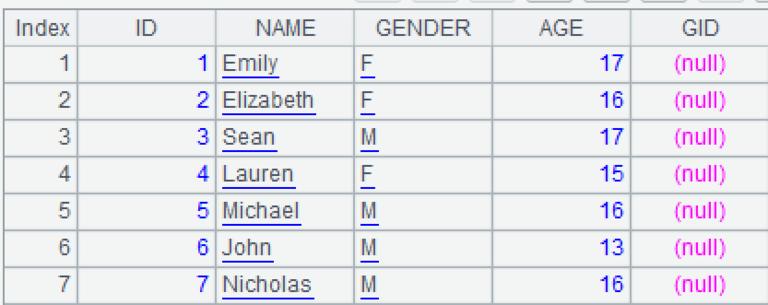
Example 1: There is a student list of a certain class, the task is to divide the class into multiple groups for doing an activity, it is required to put every three students into one group as far as possible (note thatthe total number of students may not be an integer multiple of 3), and provide a new grouped student list, indicating the group number each student falls into.
There are multiple solutions to this problem. The basic solution is to put every three rows into one group sequentially, that is, put rows [1,2,3] into group 1, rows [4, 5, 6] into group 2, and so on. Script:
A |
|
1 |
=connect("myDB") |
2 |
=A1.query@x("select Name, GENDER, AGE, null as GID from students where ClassID=1") |
3 |
=A2.group((#-1)\3) |
4 |
=A3.run(~.run(GID=A3.#)) |
A2: load the original list and add a null group number field GID. If there is specific requirement, sort according to the requirement, such as by student number. If there is no requirement, sort randomly. In the case of the latter, we can use the random function of database to code: …order by rand(). If we think this function doesn’t work well in migrating data, we can use SPL’s random function that is independent of data source to code: sort(rand ()).
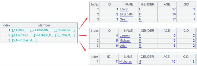
A3: group by sequence number. The groupis a grouping function, which can put the records with the same grouping key value into a group (aggregation after grouping is not necessary in this example). The symbol #represents row number, and the symbol \means taking the integer part after division, and (#-1)\3means [0,0,0,1,1,1,2]. The calculation result of A3is as follows.

A4: modify the GIDfield of each group in A3to the row number #of A3. Final calculation result:
Example 2: Divide the original list into 3 groups as equally as possible in order, that is, row numbers [1,2,3]form group 1, [4,5]form group 2, and [6,7]form group 3. The restriction condition in example 1 is the number of members of each group, while that in this example is the total number of groups. Although there is a big difference in logic, both can be easily solved in SPL.
Other codes remain unchanged, it only needs to modify the code of A3to: A2.group((#-1)*3\A2.len()).
where, the grouping key value of groupis [0,0,0,1,1,2,2]. According to the grouping rules of groupfunction, that is, the records with the same key value will be put into one group, we know that the row numbers [1,2,3]form group 1 by comparing the key values, and so on.
Alternatively, we can utilize the sequence number to implement this task. Example 3: The task is not to put adjacent records into the same group in order, but to take the record every 3 rows and put them into one group. The grouping key value is [0,1,2,0,1,2,0].
Corresponding code: A2.group((#-1)%3)
We know from the grouping rules of groupfunction that the more records there are, the more computation amount it is to compare whether the key values are equal. There are some skills for optimizing the performance, one of which is: instead of using equivalent key values as the basis for grouping, we use the group number (natural number starting from 1). In this way, the comparison of key values is avoided, and we only need to put the records with group number N into the Nth group directly.
Improve the grouping performance of example 3 by utilizing group number: A2.group@n((#-1)%3+1)
where, @nmeans direct grouping by group number, the group number is [1,2,3,1,2,3,1]. Note that example 1 and 2 are grouped by key value. Since the key value is not limited by data range, it can start from 0. If we group by group number, it must start from 1, and hence we should add 1 to the original code.
Likewise, for the example 1, we can group by group number, the performance is better: A2.group@n((#-1)\3+1)
The above examples are to calculate the group number mainly based on row numbers. In fact, group number can also be calculated based on conventional fields. For example, when the grouping field is month, we can first convert the month to a natural number, and then group by group number, which will not be detailed here.
Sort by sequence number
In some special scenarios, sequence number will participate in sorting. Since SPL provides comprehensive support to sequence number, it is more convenient to implement sorting.
Example: there is an xls table, which stores the consumption amount of each customer in the last 3 years. Here below is part of the data arranged by registration time of customers:

The task is to sort the above data by the importance of customers. The importance is related to the consumption amount and the ranking (row number) of registration time. Solution: average annual consumption + (total number of customers - row number)*10
SPL code:
A |
|
1 |
=T("d:/ClientAmount.xlsx") |
2 |
=A1.sort@z([Amount2020,Amount2021,Amount2022].avg()+(A1.len()-#)*10) |
A2: the function sort can sort records by expression; the row number #, as the retained field name, can participate in the calculation of expression directly; @zrepresents reverse order.

Align by sequence number
Alignment calculation related to sequence numbers is usually more difficult. For example, if the record set field is composed of discontinuous natural numbers, then they need to be aligned as continuous natural numbers for calculation. After alignment, each natural number may correspond to one record, multiple records, no value, etc., it is difficult for conventional computing languages to implement such alignment with missing value. SPL provides support to sequence number, and can simplify such problems.
Example 1: A community is repairing its 29 old apartment buildings numbered in natural number, and the completion progress varies from building to building. The following database table records the cost of buildings that have been repaired, and doesn’t record the cost of buildings that have not been repaired.
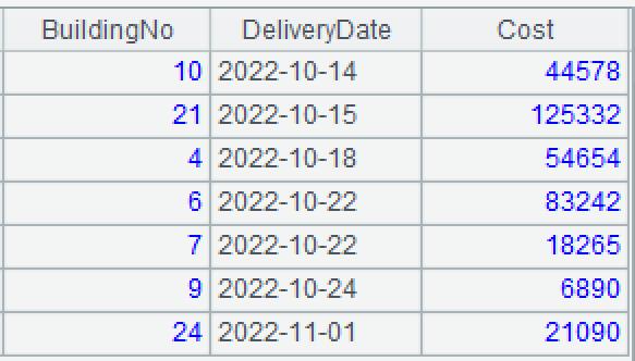
Requirement: enter a building number to query the cost of repairing the building. If a building is under repair, the cost is null.
SPL code:
A |
|
1 |
=connect("myDB").query@x("select * from BuildingRepair") |
2 |
=A1.align(29,BuildingNo) |
3 |
=A2(arg_No).Cost |
A2: align the records of building repair table to a sequence containing all building numbers. The function align()aligns the BuildingNofield of A1 to thenatural number sequence from 1 to 29.
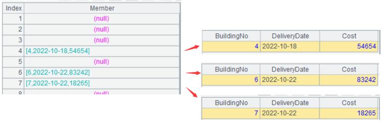
A3: query the alignment result, and the arg_Nois an external parameter. When arg_No=4, the result is 54654, and when arg_No=5, the result is null.
Itcan be seen that there is certain relationship between alignment and sorting. Alignment is equivalent to special sorting by a custom order, and there may be null record in the sorting result. With this feature, we can implement some sorting tasks that are difficult to implement in conventional methods.
The alignment result in example 1 is a single record. Sometimes, however, it may be a record set (multiple records). Example 2: A file stores a year's orders (note that orders are not available every month). Now we want to count the order amount of each month. If there isn't order in a certain month, then the order amount of this month is displayed as null. SPL code:
A |
|
1 |
=T("d:/Orders2019.txt") |
2 |
=A1.align@a(12,MONTH) |
3 |
=A2.new(#:mon,~.sum(AMOUNT):amt) |
A1: load the file. Note that there is no record in certain months.
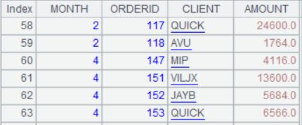
A2: align the MONTHfield of A1by a natural number sequence 1-12. The function align@a()means aligning the orders by the members of the first parameter, and each member corresponds to a group of order records. Note that the alignment result contains the month whose order is empty.
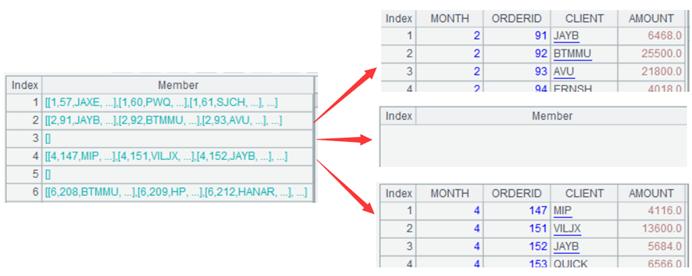
A3: generate a new table sequence based on A2, the monfield is taken from the row number (month) of A2, and the amtfield is taken from the sum of the AMOUNTof each group of orders.

If the values of MONTHfield in this example contain 12, then A2can also be written as A1.group@n(MONTH), for the reason that align@a(12)is to align by the value and position of each member from 1 to 12, if the values of MONTHcontain 12, then the group number of A1.group@n(MONTH)is also 1-12, and the missing group will be completed. Similarly, Example 1 can also be rewritten as group@n(BuildingNo).
Associate by sequence number
Usually, conventional association calculation utilizes hash algorithm to search for data. If the foreign key value is exactly the sequence number, then we can use location search with higher performance to associate record. Unfortunately, SQL does not have such concept, it still needs to calculate hash value even if it is already known that the association key is sequence number. In contrast, SPL provides support to sequence number, allowing us to associate directly by sequence number.
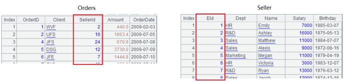
Example 1: The SellerIdof the fact table Orders.txt is the foreign key, corresponding to the primary key EId of the dimension table Seller.txt, and EIdis the natural number. Now we want to associate the two tables, and group and aggregate. SPL code:
A |
B |
|
1 |
=Orders=T("d:/Orders.txt") |
=Seller=T("d:/Seller.txt") |
2 |
=Orders.join(SellerId,Seller:#,Name,Dept) |
|
3 |
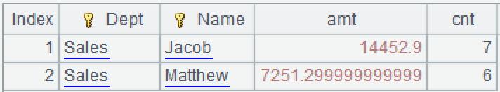
=A2.groups(Dept,Name;sum(Amount):amt,count(1):cnt) |
A1, B1: read the fact table and the dimension table. Note that the EIdfield of dimension table is natural number whose value is equal to row number #.
A2: associate by row number, and add the Nameand Deptfields of Sellerto Orders. The association field of Sellerin the joinfunction is the row number #. The association process is as follows. Taking a closer look at the Sellerrecords with Eid2 and 7 will help understand the association process.
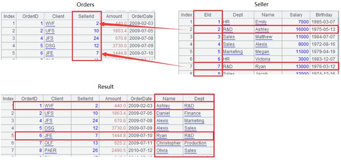
A3: group and aggregate

The primary key of the above dimension table is exactly the natural number, we can associate directly by sequence number. If the primary key of dimension table is not natural number, we can rearrange data first, and then utilize sequence number to implement high-performance association. Of course, the premise of rearranging data is that it does not affect business logic.
Example 2: The foreign key Client of Ordersand its corresponding primary key IDof Customerare both strings:
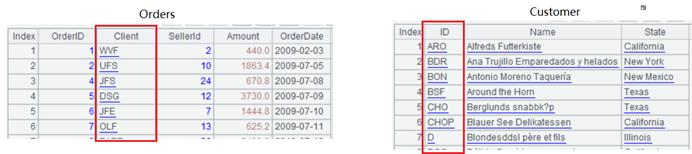
Rearranging process: replace the Clientof Orderswith the row number corresponding to the IDof Customerin advance, and dimension tables like Customerusually do not need to be changed. Once association is performed later, we can utilize the row number to associate as long as the row numbers of the records in Customerremain unchanged. Keeping the row numbers unchanged is easy. To be specific, if the data source is a database, just sort by fixed field; if the data source is a file, just take out the data by the order in file directly.
SPL code for data rearranging or preprocessing:
A |
B |
|
1 |
=Orders=T("d:/Orders.txt") |
=Cust=T("d:/Customer.txt") |
2 |
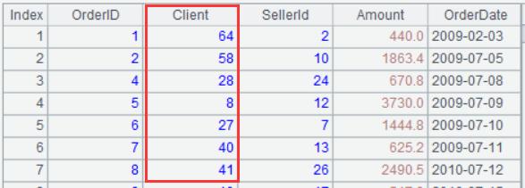
=Orders.join(Client,Cust:ID,# : Client) |
|
3 |
=file("d:/OrdersS.btx").export@b(A2) |
A2: associate the IDfield of Custwith the foreign key Clientof Orders. After association, only fetch the row number #of Custand name it Clientso as to replace the original Clientfield of Orders.
A3: store the rearranged Ordersin any format. Here, it is stored in SPL’s btxfile, which has better read/write performance.
At this point, we can continue to utilize sequence number to implement high-performance association calculation, and the code logic remains unchanged.
In this example, conditional filtering on the dimension table is not performed, mainly because the scenario of filtering dimension tables is not suitable for associating directly by sequence number. Specifically, filtering first and then associating will cause the row numbers of dimension table to change, which in turn results in an error in association, while associating first and then filtering is equivalent to filtering the fact table, it will result in poor performance since the fact table is usually large. To solve this problem, we can utilize the aligned sequence to perform indirect sequence number association. This method can not only implement the operation equivalent to filtering dimension table while keeping the sequence numbers unchanged, but it can also implement high-performance association on large fact table.
The aligned sequence refers to a sequence with the same length as dimension table, and each member of sequence indicates whether the dimension table record at the corresponding position meets the filtering condition. The record that meets the condition is true, otherwise it is false. Let's now see an example.
Example 3: The data, association relationship, and aggregation calculation in this example are the same as those in Example 1, the differences are that the Ordersin this example is too large to be stored in memory, and it is required to filter the small dimension table Seller.txt.
SPL code:
A |
B |
|
1 |
=Orders=file("d:/Orders.btx").cursor@b(SellerId,Amount) |
=Seller=T("d:/Seller.txt") |
2 |
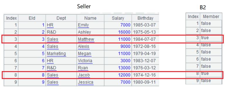
=Seller.(["HR","Sales"].contain(Dept) && Salary>10000) |
|
3 |
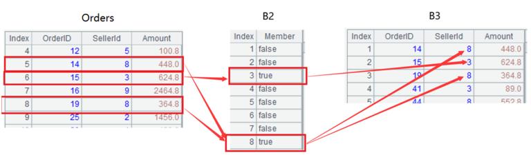
=Orders.select(B2(SellerId)) |
|
4 |
=B3.groups(Seller(SellerId).Dept,Seller(SellerId).Name;sum(Amount):amt,count(1):cnt) |
A1, B1: load data. Use cursor to retrieve the large fact table. In order to improve performance, only fetch 2 involved fields.
B2: perform conditional filtering on the dimension table to generate an aligned sequence.
B3: filter the fact table with the aligned sequence to filter out the records that meet the conditions. When performing location search by employee number (i.e., the row number of dimension table) to get the member of B2, we can know whether the employee meets the conditions, such as B2(5)=false, B2(8)=true. In the selectfunction, if the parameter value is true, then it means this record is selected. Note that because the fact table is cursor, the filtering in this step will be delayed until grouping and aggregating, and hence the filtering result is not immediately visible here. When filtering is executed later, the filtering process will be as follows:
B4: group and aggregate the filtered fact table. The Seller(SellerId).Deptis used to fetch the Deptfield of dimension table, which is actually an association action. Calculation result:
SPL Official Website 👉 http://www.scudata.com
SPL Feedback and Help 👉 https://www.reddit.com/r/esProc
SPL Learning Material 👉 http://c.scudata.com
SPL Source Code and Package 👉 https://github.com/SPLWare/esProc
Discord 👉 https://discord.gg/ydhVnFH9
Youtube 👉 https://www.youtube.com/@esProc_SPL


Chinese version