

Ordered storage of SPL
Ordered storage is to write the data into external storage (mainly refers to the hard disk) continuously after sorting them by some fields (usually refer to the primary keys or part of primary keys). Not only can the ordered storage achieve low-cost data compression, but it can also avoid reading the hard disk in a frequent jumping manner. Moreover, since the data continuously read from hard disk during calculation are already ordered, it can implement high-performance algorithms designed specifically for ordered data, such as the binary search, fast filtering, ordered grouping, ordered association. In this article, we will introduce the principle of SPL’s ordered storage in detail.
Storage structure
SPL composite table supports two storage ways: row-based storage and columnar storage. As for which method to use, programmers should choose according to actual scenario. The source data are usually written into the composite table in batches, and each batch contains a certain number of records. Since the composite table that adopts the row-based storage also stores the data continuously by records, SPL only needs to write each batch of source data into composite table file in sequence by records. In this way, it just needs to read the records in sequence when calculating. The code to generate the row-based storage composite table is roughly like this:
file("T-r.ctx").create@r(#f1,#f2,f3...).append(cs)
//Create the row-based storage composite table, and write the data from the cursor cs into composite table. f1 and f2 are preceded by #, indicating that the two fields are in order. The ordered fields are specified explicitly here to facilitate the use of ordered characteristics when coding.
Unlike the row-based storage, the columnar storage essentially stores the same fields of each record together, and different fields are stored in different areas. If two or more fields are involved in calculation, these field values need to be found respectively and combined before use. When generating a columnar storage composite table, SPL first divides it into the data blocks with a certain size, and each block only stores the data of the same field. Then, write the field values of each batch of source data into the data block of the corresponding field respectively. When a data block is filled with a certain field, it needs to skip the data block that has stored other fields, and generate a new data block so as to continue storing the data of this field. The start and end positions and size of these data blocks will not change with the data appending.
Suppose that the data table has m fields F1 to Fm, the formed columnar storage composite table is roughly as follows:

In this figure, block#k represents the kth data block. A field is stored contiguously in the same data block. However, when this field occupies multiple data blocks, these blocks are often discontinuous. For example, the field F1 in the figure is continuous in the data block block#1, but the next data block that stores F1 is not block#2 but block#x. Although the two blocks that store F1 are not continuous, frequent random reading of hard disk can be avoided as long as each data block is large enough. For the mainstream hard disks, when the storage capacity of data block exceeds 1M, the proportion of jumping cost will be very small, and it can be considered that each field is logically continuous.
After the ordered fields of columnar storage composite table are stored continuously, the values of adjacent fields are highly likely to be the same. In this case, SPL only needs to store one value and the number of repetitions, and does not need to store the same value multiple times, which effectively compresses the data and saves a lot of storage space.
The SPL code to generate the columnar storage composite table is as follows:
file("T-c.ctx").create(#f1,#f2,f3...).append(cs)
//Create the columnar storage composite table, and write the data from the cursor cs into composite table. Likewise, # indicates the fields following it are ordered. Although the code is simple, it encapsulates the above algorithms such as blocking, columnar storage ordered compression.
SPL composite table does not check whether the fields are in order when appending the data. Thus, the programmer needs to ensure that the written data are indeed in order.
After the data are orderly stored, the ordered characteristic can be utilized to implement high-performance algorithms such as the common binary search. SPL code for binary search is also very simple:
= file("data.ctx").open().find(123456)
//Open the composite table, and utilize the binary search to search for the records with primary key value of 123456.
Another example: interval conditional filtering. The header of composite table file records the start position of data blocks. When filtering the ordered fields, the records can be directly taken according to the start position. To judge whether there is a search target in a block, we can compare the values of ordered field in the records through the filter conditions and the ordered characteristic. If a target valve is not found, skip this block directly. In this way, the amount of data to be read can be reduced and the computing time can be saved.
= file("data.ctx").open().cursor(f1,f2,f4;f1>=123456 && f1<234567)
//Open the composite table, and perform the interval search by the ordered field f1.
A small amount of modifications
After generating the stored data, there may be data change operations, including insertion, deletion and modification. To ensure high performance, these operations cannot be performed directly on the composite table for reasons: the modified new value is not necessarily as same size as the original value, and thus the data cannot be directly replaced in the original position; the composite table does not reserve blanks for inserting the data, and deletion of data will cause data discontinuity. Although we can implement data changes by rewriting the composite table, it needs to re-sort to maintain ordered storage, and it also needs to regenerate the composite table, it will take a long time.
For composite table with primary key, SPL provides the supplementary area mechanism to implement a small amount of data changes. That is, a separate supplementary area (as shown in the figure below) is set in the composite table file to store the changed data.
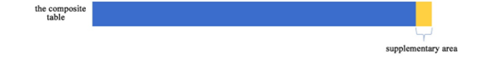
When reading this composite table, the data in the supplementary area (yellow part) and the normal data (blue part) are merged together for calculation.
The code for data change operation is roughly as follows:
| A | B | |
|---|---|---|
| 1 | =file(“data.ctx”).open() | |
| 2 | =10.new(rand(1000):ID,…) | >A1.update(A2) |
| 3 | =10.new(rand(10000):ID,…) | >A1.delete(A3) |
| 4 | //A2 and A3 simulate the data waiting to be modified and deleted with random record sequence. | |
The supplementary area mechanism can complete the data change operation in a very short time, and can also ensure the orderliness of the read data. Moreover, the complement area is transparent to the SPL programmer, and the syntax remains unchanged.
Only when the data changes a little, the supplementary area has little impact on the performance. After multiple modifications, however, the supplementary area will get larger and larger, and the impact on performance will be greater. Therefore, the supplementary area needs to be cleaned up regularly by merging it into original data area, and cleared.
| A | B | |
|---|---|---|
| 1 | =file(“data.ctx”).open() | |
| 2 | if (day(now())==1 | >A1.reset@q() |
| 3 | //Clean up the supplementary area on the 1st of every month. |
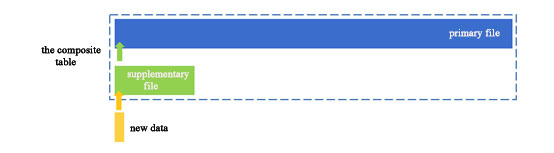
The following figure briefly describes the method of using reset@q to clean up the supplementary area:

Assume that the data are stored in ascending order by primary key. In the figure, SPL first determines the minimum primary key value in the supplementary area, and then finds this value in the normal data, that is, the position of the yellow arrow. The normal data (blue part) preceding the position remain unchanged, and rewrite the composite table starting from the position. In this way, it not only ensures the ordering by primary keys, but also reduces the amount of data to be rewritten and saves the time.
Regular appending of data
For some ordered data, insertion, deletion or modification will not occur, but the new data will be appended continuously, sometimes it cannot be appended directly at the end of the original data. For example, the order composite table is stored in order by the user ID for the convenience of user-related counting; however, the new order data are usually ordered by time, and the time is later than the data in the composite table; since the user IDs still remain unchanged, direct appending will destroy the order of the user IDs. If the big sorting was performed on the new data together with the original data, followed by regenerating the composite table, it would take a long time.
In this case, we can divide the data composite table file into two parts: the historical data composite table hisdata.ctx and the incremental data composite table newdata.ctx. Every time the data are appended only on the incremental data composite table. After a period of time, merge the new data with historical data. The specific method can be roughly represented by the following figure:
Having sorted the new data by the ordered fields of historical data composite table, orderly merge new data with the incremental data composite table. In this way, each time we only need to merge and sort the new data with the incremental data composite table, hereby greatly reducing the amount of involved data. When reading the composite tables, the data will be read from two files respectively, and then merged to obtain a result set. The result set is still in order. Although doing so will slightly affect the performance compared with accessing a single file, it can still take advantage of the ordered characteristic.
Unlike the supplementary area, this way has little impact on the access performance even if the incremental data composite table becomes large over time. However, too large incremental data composite table will slow down the speed every time the data are appended. Therefore, it is necessary to merge on a regular basis to form a larger composite file, and then empty the incremental data composite table. For example, the new data of every day are merged into the incremental data composite table, and merge the two composite table on the 1st day of each month. SPL code:
| A | B | |
|---|---|---|
| 1 | =file("data.ctx").open() | |
| 2 | =file("data_new.btx").cursor@b() | |
| 3 | if (day(now())==1 | >A1.reset() |
| 4 | >A1.append@a(A2) |
Before reading data, it needs to merge the historical data composite table with the incremental data composite table, for example:
=[file("hisdata.ctx").open().cursor(),file("newdata.ctx").open().cursor()\].merge(#1)
It should be noted that the cursor sequence should be in the same order as the data files, that is, [historical data, incremental data].
Bulk deletion
The composite table ordered by date may cause a large amount of data to expire. For example, the data of historical table are ordered by fields such as date, and this table stores the data of 10 years after 2010. By the year 2014, the data in 2010 are out of date and need to be deleted. The data, however, are ordered by date, and deleting them will cause the whole composite table to be rewritten, which is very time-consuming.
SPL provides the multi-zone composite table, which can quickly and conveniently delete expired data. The multi-zone composite table is a composite table composed of multiple files, and such files are called the zone of the table. Since SPL uses different zones to store data of different dates, when the data stored in a certain zone expires, just directly delete the corresponding file. The multi-zone composite table mechanism can be illustrated by the following figure:
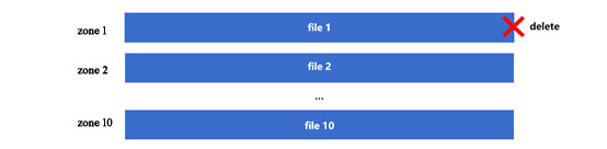
When the data in zone 1 is out of date, delete file 1 directly. When opening the composite table again, don’t add zone 1, and there is no need to rewrite the data in other zones. The corresponding code is roughly as follows:
| A | |
|---|---|
| 1 | =file(“data.ctx”:to(10)).create(#dt,…;year(dt)-2009) |
| 2 | =file(“data.ctx”:to(2,10)).open() |
A1 creates the composite table and sets 10 zones, namely zone 1, 2, …, 10. The year(dt)-2009 is the zone number expression, which means that the data are divided into different zones by the year. When using the option append@x to append data, SPL will calculate year(dt)-2009 for each appended record, and append the data into the file with corresponding zone number according to the calculation result. If zone 1 is deleted, just open zones 2 to 10 when opening the composite table in A2.
Deleting the expired data using multi-zone composite table is to delete file in fact, which is very fast. If not using the multi-zone composite table, it would need to rewrite all remaining data. Even if the data are already ordered by date and there is no need to re-sort, it is still very time-consuming to rewrite them all. Of course, we can also manually create several composite table files to make each table store the data of a time period, and then concatenate multiple files during calculation, which is exactly the idea of multi-zone composite table. However, the code will be complex in doing so. In contrast, the multi-zone composite table encapsulates these processes, and the code is simpler.
SPL Official Website 👉 http://www.scudata.com
SPL Feedback and Help 👉 https://www.reddit.com/r/esProc
SPL Learning Material 👉 http://c.scudata.com
SPL Source Code and Package 👉 https://github.com/SPLWare/esProc
Discord 👉 https://discord.gg/ydhVnFH9
Youtube 👉 https://www.youtube.com/@esProc_SPL


Chinese version