SPL Simplified SQL - Multilevel Join
In the development of database application, we often need to face complex SQL computing, and multilevel join is one of them. The join statement of SQL is relatively abstract and only suitable for expressing simple association. Once there are more levels of association, the corresponding code will become very complex. SPL can use object references to express join relationships, which makes the code more intuitive. Here is an example to illustrate.
Table channel stores the corresponding relationship between all channels and their superior channels of a website, which is represented by ID and PARENT fields, up to four levels, in which root represents the website itself (that is, the root node). Some of the data in the table are as follows:
ID |
PARENT |
NAME |
p1 |
root |
news |
p2 |
root |
health |
p3 |
root |
manage |
c11 |
p1 |
Scenic Introduction |
c12 |
p1 |
Places of Interest |
c13 |
p1 |
Local culture |
c21 |
p2 |
Scenic Service |
c22 |
p2 |
E-commerce |
c31 |
p3 |
Travel Tips |
d111 |
c11 |
Investment Projects |
d112 |
c11 |
Virtual tour |
d113 |
c11 |
Places of Interest |
d114 |
c11 |
Historical legends |
d115 |
c11 |
Resort weather |
d121 |
c12 |
Ticket booking |
Now we want to list the names of all the subordinates of the channel hierarchically according to the ID input by the parameters, separated by commas between the subordinates of the same layer. Assuming that the value of the parameter arg1 is p1, the expected result is shown in the following figure:

SPL codes are as follows:
A |
B |
|
1 |
=db.query("select * from channel") |
>A1.switch(PARENT,A1:ID) |
2 |
=create(ID,LEVEL,SUB) |
|
3 |
=A1.select(PARENT.ID==arg1) |
>A2.insert(0,arg1,1,A3.(NAME).string()) |
4 |
=A1.select(PARENT.PARENT.ID==arg1) |
>A2.insert(0,arg1,2,A4.(NAME).string()) |
5 |
=A1.select(PARENT.PARENT.PARENT.ID==arg1) |
>A2.insert(0,arg1,3,A5.(NAME).string()) |
6 |
>file("channel.xlsx").xlsexport@t(A2) |
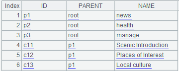
A1: Query table channel, and part of the result is as the following figure:
B1:>A1.switch(PARENT,A1:ID), Use the function switch to replace the PARENT field in the table with the corresponding record reference, as shown in the following figure:
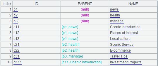
After switching, PARENT. ID can be used directly to represent the parent channel, while PARENT. PARENT. PARENT. ID can directly represent the upper three level (Great Grandparent) channels. Although join can also be used to represent this self-connection in SQL, it is obviously easy to cause confusion when there are more levels.
A2:=create(ID,LEVEL,SUB), Create an empty table to store the final calculation results.
A3:=A1.select(PARENT.ID==arg1), Look up the records whose parent channel is equal to the parameter arg1 from the table, that is, the lower level (sub) channel of arg1. The results are as follows.

B3:>A2.insert(0,arg1,1,A3.(NAME).string()), Add a record to A2, the first field value is arg1; the second field value is 1, representing the first level subchannel; and the third field is the expression A3.(NAME).string(), indicating that the column NAME in A3 is taken out and spelled into comma-separated strings. The results are as follows.

A4:=A1.select(PARENT.PARENT.ID==arg1), this code is similar to A3, Look up the lower two level channels of arg1 channel from the table. The results are as follows:
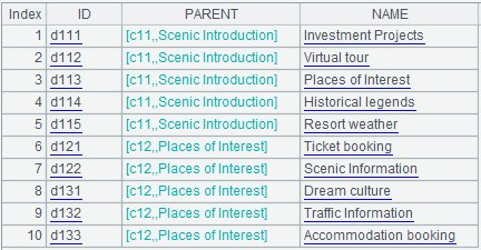
The code of A5 is similar to A4, Select the lower three level channels of arg1 channel. Similar methods can be used to easily select the lower N-level channels.
The code of B4 and B5 is similar to B3, add new records to A2, only the level field is changed to 2 and 3. After executing B5, A2 is the final result of this calculation.

Just now the value of arg1 is p1. If C12 is input, the result is as follows:

Sometimes we want to see clearer data, such as listing all the subordinate channels of a channel one by one, and marking out hierarchical relationships. As shown in the following figure:
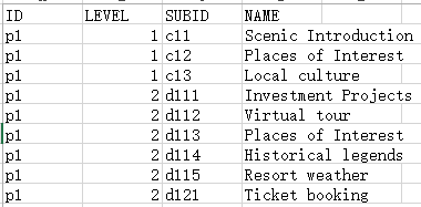
To implement this algorithm, we can use the following code:
A |
B |
|
1 |
=db.query("select * from channel") |
>A1.switch(PARENT,A1:ID) |
2 |
=create(ID,LEVEL,SUB) |
|
3 |
=A1.select(PARENT.ID==arg1) |
=A2.insert(0,arg1,1,A3) |
4 |
=A1.select(PARENT.PARENT.ID==arg1) |
=A2.insert(0,arg1,2,A4) |
5 |
=A1.select(PARENT.PARENT.PARENT.ID==arg1) |
=A2.insert(0,arg1,3,A5) |
6 |
=A2.(~.SUB.new(A2.ID,A2.LEVEL,ID:SUBID,NAME)) |
|
7 |
=A6.union() |
The red font is the changed code, of which the B3 code is =A2.insert(0,arg1,1,A3), indicating that the records of A3 are stored directly in A2. Assuming that the value of arg1 is p1, the results are as follows:

Click on the SUB field to see the detailed records:

As you can see, the field value of SPL is generic and can store record group or single record. The essence of function switch is to switch the foreign key to the corresponding record in the main table.
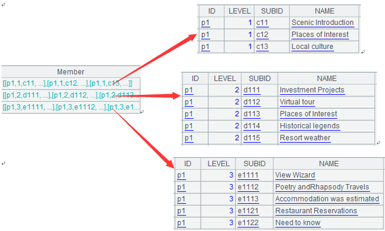
After executing B5, the results in A2 are as follows:

A6:=A2.(~.SUB.new(A2.ID,A2.LEVEL,ID:SUBID,NAME)), Spell the ID and LEVEL in A2 into each record in the SUB field. Among them, A2.() denotes the calculation of A2, in which "~" can be used to represent each record in A2, and ~. SUB denotes the SUB field (record group) of each record. Function new is used to generate a new table, namely: ID field in A2, LEVEL field in A2, ID field in SUB, NAME field in SUB. When the calculation is completed, the values of A6 are as follows:
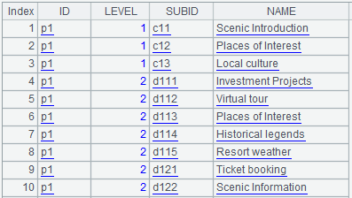
A7=A6.union(), this code is used to piece together the records of A6 to form the final calculation result:
Sometimes we need to list all the subordinate channels of each channel directly. To implement this algorithm, we can use the SPL for statement with the following code:
A |
B |
C |
|
1 |
=db.query("select * from channel") |
>A1.switch(PARENT,A1:ID) |
|
2 |
=create(ID,LEVEL,SUB) |
||
3 |
for A1.(ID) |
=A1.select(PARENT.ID==A3) |
=A2.insert(0,A3,1,B3) |
4 |
=A1.select(PARENT.PARENT.ID==A3) |
=A2.insert(0,A3,2,B4) |
|
5 |
=A1.select(PARENT.PARENT.PARENT.ID==A3) |
=A2.insert(0,A3,3,B5) |
|
6 |
=A2.(~.SUB.new(A2.ID,A2.LEVEL,ID:SUBID,NAME)) |
||
7 |
=A6.union() |
The code for A1.(ID) in A3 indicates that loop the ID field of A1. Each time one item is taken out, and the loop variable can be represented by the cell A3 where the loop statement is located. The scope of the loop can be expressed by indentation, and the scope of the loop in the example is B 3:C5. The final calculation results are in A7. Some of the data are as follows:
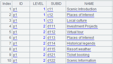
From these examples, we can see that when using SPL to simplify multi-level Join problems, the idea is intuitive and clear, the code is simple and easy to understand, and the hierarchical relationship is clear. Compared with SQL, such SPL code can greatly reduce the development cost, and greatly simplify the post-optimization and maintenance work.
SPL Official Website 👉 https://www.scudata.com
SPL Feedback and Help 👉 https://www.reddit.com/r/esProcSPL
SPL Learning Material 👉 https://c.scudata.com
SPL Source Code and Package 👉 https://github.com/SPLWare/esProc
Discord 👉 https://discord.gg/2bkGwqTj
Youtube 👉 https://www.youtube.com/@esProc_SPL


