In the article “the whole process of using historical data to make business prediction” (hereinafter referred to as the previous article), we introduced how to use historical data to make business prediction. Different business needs will have their own particularity. For example, in many business scenarios, there is a phenomenon of data imbalance, such as bank loan default, only a small number of people default; insurance fraud, fraudsters are also individual phenomena; there are also the proportion of defective products in product quality, and the phenomenon of unplanned parking in industrial production… The occurrence rate of these rare phenomena is very low, but once it occurs, it will cause great losses, so we should try our best to predict and avoid them. This article will introduce how to predict these rare phenomena.

1. Prepare historical data

The process of data preparation is as described in the previous article, but for this scenario where rare phenomena need to be predicted, data imbalance should be considered. We call the records of rare phenomena in historical data as positive samples. Data imbalance means that positive samples are too few in the total data. At this time, even if the total amount of data is large, it is difficult to build an effective model. Therefore, in the preparation of data, it is necessary to extract as many positive samples as possible. Generally speaking, the more complex the problem is, the more quantity of positive samples is needed. However, even a simple problem usually requires at least a few hundred positive samples to build a usable model. On the other hand, we can not only take positive samples. For example, in order to model and predict the default of loan users, it is necessary to ensure that the data of default customers reaches a certain number, but not all of them are the data of default customers, and the data of normal customers should also be collected.

2. Build the model

As mentioned in the previous article. For unbalanced data sets, YModel will automatically sample to balance the proportion of positive samples and negative samples (i.e. normal samples). Users do not need to operate by themselves. However, we can modify and set the required trim ratio, as shown in the figure below. For beginners, it is generally recommended to adopt the default scale.

3. Predict

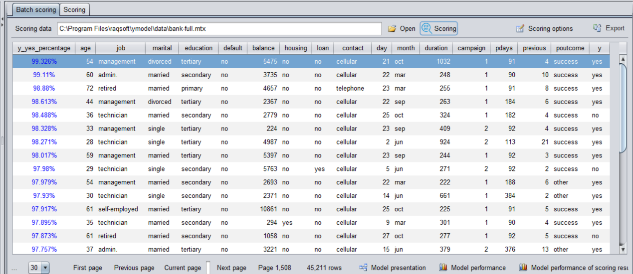
After the first two steps of processing, the established model can realize the prediction. Similarly, it is sorted from high to low according to the predicted probability, and it is OK to find the customers or samples with higher probability in front to focus on the investigation. The top samples are more likely to have rare phenomena.

4. Recall index

In the scenario of unbalanced data distribution, it is meaningless to only check the prediction accuracy. What is more meaningful to us is recall rate. Recall represents how many of the positive samples are correctly predicted. For an exaggerated example, there are only 5 terrorists out of 1 million people in the airport, because terrorists are very few. If the accuracy rate is used to evaluate the model, the accuracy of 99.9995% can be achieved as long as all the people are identified as normal people. But obviously this doesn’t make sense, no terrorist would be caught. That is to say, although the accuracy of this model is very high, the recall rate is 0 / 5 = 0. On the contrary, the other model predicted that 100 people would be high-risk group, and all five terrorists were included in the 100 people. At this time, the accuracy rate was reduced to 99.9905% (95 people were wrong), but the recall rate was 5 / 5 = 1, and all the terrorists were caught. Such a model would make more sense.

In YModel, we will use the recall curve to judge the recall rate. As shown in the figure below, the abscissa represents the number of the predicted probability of rare occurrence in order from high to low, 10,20…represents the top 10%, 20%… of the samples, and the ordinate represents the recall value corresponding to each ranking stage. The recall rate corresponding to the abscissa 10 in the figure is about 0.75, indicating that 75% of the rare phenomena can be captured in the top 10% of the predicted probability. That is to say, compared with screening all the samples, we can find 75% of the rare (abnormal) cases with 10% of the workload. The closer the recall curve is to the upper left corner, the better the ability of the model to capture rare phenomena (default, fraud, defective products, abnormal equipment…).