Convert row-style table and cross table
Example 1: Row-style to cross
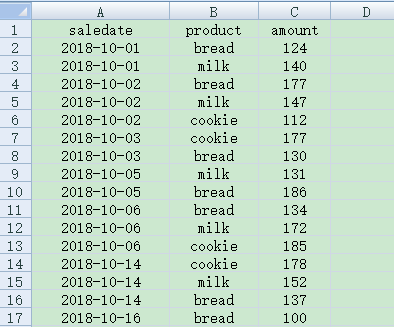
There is a daily sales record table sales.xlsx, some of the data is shown in the figure below:

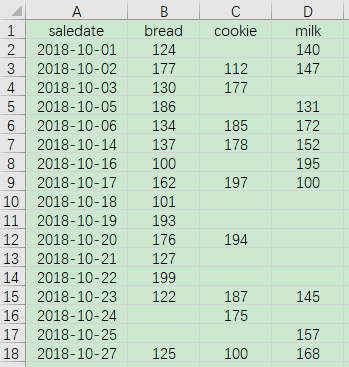
Make a cross-statistical table with date as the left header and product as the upper header, as shown in the figure below:

Write SPL script:
A |
|
1 |
=T("E:/work/sales.xlsx") |
2 |
=A1.pivot(saledate;product,amount) |
3 |
=T("E:/work/sales1.xlsx",A2) |
A1 Read in the sales.xlsx file
A2 Group A1 with saledate, row to column, product value is converted to new column name, amount value is new column value.
A3 Save A2 to the file sales1.xlsx
Example 2: Cross to row-style
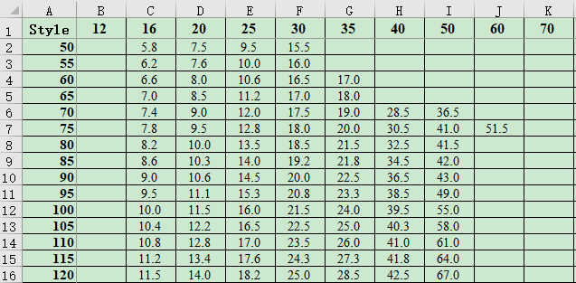
The Excel file book1.xlsx has the cross-tab data shown in the figure below. The column direction is the width of the product specification, and the row direction is the length:

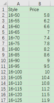
Turn the data into a row-style table, and the specifications are displayed as width * length, as shown in the following figure:

Write SPL script:
A |
|
1 |
=T("E:/work/book1.xlsx") |
2 |
=A1.pivot@r(Style:length;width,Price) |
3 |
=A2.select(Price).sort(width,length).new(width/"*"/length:Style,Price) |
4 |
=T("E:/work/book2.xlsx",A3) |
A1 Read in the book1.xlsx file
A2 Group A1 by Style, column to row, and name the new column length at the same time, option @r means column to row, the original column name is converted to the value of the new column width, and the original cross grid value is converted to the new column Price value.
A3 Select the records whose price Price is not empty from A2, and then sort them by width and length, then create a new data set, use width, asterisk and length as the value of the new column Style, and select the Price column at the same time.
A4 Save A3 to the file book2.xlsx
SPL Official Website 👉 https://www.scudata.com
SPL Feedback and Help 👉 https://www.reddit.com/r/esProc_Desktop/
SPL Learning Material 👉 https://c.scudata.com
Discord 👉 https://discord.gg/2bkGwqTj
Youtube 👉 https://www.youtube.com/@esProcDesktop
Linkedin Group 👉 https://www.linkedin.com/groups/14419406/


