SPL Programming - 10.4 [Association] Join
Let’s continue to see the above order example. After picking out the records with the same order number but different contents in the two files, we want to spell the fields (except the order number) together and compare them. That is to form a data table with twice the number of fields (except the order number).
We usually use the join() function to accomplish this task.
| A | B | |
|---|---|---|
| 1 | =T(“data1.xlsx”) | =T(“data2.xlsx”) |
| 2 | =[A1,B1].merge@i(ID) | =[B1,A1].merge@i(ID) |
| 3 | =join(A2:a,ID;B2:b,ID) | |
| 4 | =A3.new(a.ID:ID,a.Company:CompanyA,b.Company:CompanyB,a.Area:AreaA,b.Area:AreaB,a.OrderDate:OrderDateA,b.OrderDate:OrderDateB,a.Amount:AmountA,b.Amount:AmountB, a.Phone:PhoneA, b.Phone:PhoneB) | |
The join() function of A3 returns a table sequence with two fields, a and b respectively. It will concatenate the records in A2 and B2 according to the ID field value, that is, fill the A2 record and B2 record with the same ID into field a and field b respectively as a record in the returned table sequence. The value of field a or field b is also a record, which is a bit like the result of a foreign key being switched. After we understand the calculation result of A3, although A4 is long, it is easy to understand.
Unlike merge(), the task of join() is often to make the data table wider, and merge@u will make the data table longer (more records).
A bigger difference from merge()is that the data tables targeted by merge() are generally of the same data structure. While the common scenario of join()is two (or more) data tables with different data structures.
Let’s continue to use the personnel table generated earlier, we now have a personnel table with gender, height and weight, as well as an employee table with nationality and department. We want to make the two tables into a wider table. If the name field of the personnel table is the same as the eid field of the employee table, it means that it is the same person.
Let’s sort out the code used to generate data. We don’t use the department table at the moment, just discard it.
| A | B | C | |
|---|---|---|---|
| 1 | =100.sort(rand()) | [HR,R&D,Sales,Marketing,Admin] | [CHN,USA] |
| 2 | =100.new(A1(#):eid,C1(rand(2)+1):nation,B1(rand(5)+1):dept) | ||
| 3 | =100.new(string(~):name,if(rand()<0.5,“Male”,“Female”):sex,50+rand(50):weight,1.5+rand(40)/100:height) | ||
The eid in employee table A2 is disordered.
Let’s finish the task:
| A | B | C | |
|---|---|---|---|
| … | … | ||
| 4 | =join(A3:P,int(name);A2:E,eid) | ||
| 5 | =A4.new(P.name,P.sex,P.weight,P.height,E.nation,E.dept) | ||
Because the name of A3 is a string type, which is different from the eid of A2, it needs to be converted and written as int(name). We can also convert A2 and write A4 as:
=join(A3:P,name;A2:E,string(eid)) .
The calculation result of A4 is as follows:
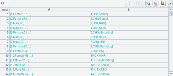
A table sequence with two fields. The field values are A3 record and A2 record respectively. Because we did not set the primary key for A2 and A3, the development environment will display the fields of the record as a sequence. It can be seen that the first field of the records on the left and right sides of the same line, that is, name and eid, are the same. This is the result of the join()operation. It will spell together the records with the same name in A3 and eid in A2 (Actually, int(name) and eid are the same, but they look the same).
Then A5 can easily get the desired results, which will not be explained in detail.
Two data tables can generate a data table with two fields through the equal relationship between certain fields (or expressions). Based on this new data table, the fields of two original data tables can be referenced for operation at the same time, so as to complete the association of the two tables. The field (expression) used to determine association is called association key, and records with equal association key values are called associated records. This association operation is called join.
The foreign key association mentioned in the previous section is also a join operation. It uses the foreign key of the fact table and the primary key of the dimension table as the association key. However, we rarely express the operation result of foreign key association as a table sequence using two fields with records as values as a data structure. Instead, we are used to using the previous method to switch the foreign key with the switch()function or spell the dimension table fields into the fact table with join() (not the join() we are talking about).
If we already set the primary key for A2 and A3 tables, we do not need to write the association key during join().
| A | B | C | |
|---|---|---|---|
| 1 | =100.sort(rand()) | [HR,R&D,Sales,Marketing,Admin] | [CHN,USA] |
| 2 | =100.new(A1(#):eid,C1(rand(2)+1):nation,B1(rand(5)+1):dept).keys(eid) | ||
| 3 | =100.new(~:name,if(rand()<0.5,“Male”,“Female”):sex,50+rand(50):weight,1.5+rand(40)/100:height).keys(name) | ||
| 4 | =join(A3:P;A2:E) | ||
We need to change the generation statement in A3 to directly use integers as the values of the name field, so that the primary keys of the two tables do not need a conversion and directly serve as the association key.
The join using the primary key as the association key is called the homo dimension association, and the two tables are also called the homo dimension table to each other. In database terminology, the homo dimension association is a one-to-one association, that is, a record in an association table will only be associated with one record in another association table, not multiple, because the primary key is unique.
Let’s continue with this code and change it a little bit. A2 randomly selects 80 integers between 1 and 100 as the primary key to generate 80 records; A3 directly selects 1-90 as the primary key to generate 90 records. In this way, the primary keys of A2 and A3 still have a lot in common, but they also have a small number of primary key values that the other does not have(Because of random generation, the result of each running may be different, but it does not affect our discussion).
| A | B | C | |
|---|---|---|---|
| 1 | =100.sort(rand()) | [HR,R&D,Sales,Marketing,Admin] | [CHN,USA] |
| 2 | =80.new(A1(#):eid,C1(rand(2)+1):nation,B1(rand(5)+1):dept).keys(eid) | ||
| 3 | =90.new(~:name,if(rand()<0.5,“Male”,“Female”):sex,50+rand(50):weight,1.5+rand(40)/100:height).keys(name) | ||
| 4 | =join(A3:P;A2:E) | ||
| 5 | =A4.len() | =A2.(eid)^A3.(name) | =B5.len() |
Look at the result of A4:
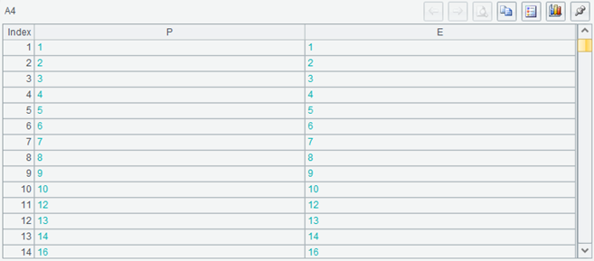
The left and right are still equal, but there are obviously missing sequence numbers (that is, primary key).
Looking at A5, of course, it will not be 100, but it is not 80 or 90, but smaller.
The join() function will find records with equal association keys in both tables to associate. If the association key value of one table does not exist in the other table, the corresponding record of this table will also be discarded. This join is called inner join. The association key set in the result of the calculated table sequence is the intersection of the association key sets of the two associated table sequences, that is, B5 in the above code, and A5 is bound to be equal to C5, which is usually less than the length of A2 or A3.
Let’s try again after changing the last two lines of code:
| A | B | C | |
|---|---|---|---|
| … | … | ||
| 4 | =join@1(A3:P;A2:E) | ||
| 5 | =A4.len() | =A3.(name) | =B5.len() |
Execute again, and then look at A4
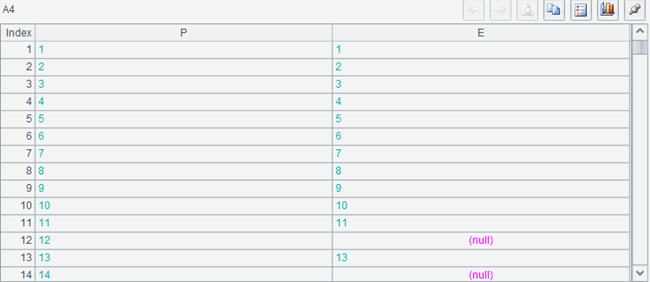
The record primary key in the values of the P field is complete, ranging from 1 to 90, and corresponds to the records of A3 one by one. Some records of the E field are filled with null. A5 is also 90, the same length as A3.
The join()with @1 will be based on the association table on the left (the first parameter). If there are records with the same association key as the left in the right table, it will be associated. If there is no record, it will be filled with null. The association key value of the result table sequence is the same as that of the left table, and its length is also the same as that of the left table.
This join based on the left is called left join.
Some database systems also have right join, that is, join based on the right. However, SPL does not provide it. It is not necessary because it can be done by swapping the parameter position.
And this @1 is the number 1, not the letter l. It means that the join() is based on the first parameter.
Continue:
| A | B | C | |
|---|---|---|---|
| … | … | ||
| 4 | =join@f(A3:P;A2:E) | ||
| 5 | =A4.len() | =A2.(eid)&A3.(name) | =B5.len() |
Then look at A4:
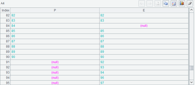
Because the primary key of A3 is from 1 to 90, the records in the front exist. Pull the table to the end, and the last few records can be seen.
Now there are null field values on the left and right sides, and A5 is greater than 90, but it is often not 100.
The join() with @f will consider both tables. If the association key value exists in either side, a record will be generated in the result table sequence. If both sides have records with association key value, the records will be filled in the corresponding field to realize association. For an association key value, if only one table has a corresponding record, fill it in the corresponding field and fill null in the corresponding field of another table. Finally, the associated key value set in the result table sequence will be the union of the associated key sets of the two table sequences involved in the association, or B5 in the code, and A5 will be the same as C5, usually greater than the length of A2 or A3.
This two-sided join is called full join.
Inner join, left join and full join are very important concepts. When performing join operation, we must make sure which kind of join to use. The results of different joins will be very different.
Foreign key association is usually left join, that is, based on the fact table. If the switch()function cannot find the associated record in the dimension table, it will fill the foreign key field with null. While switch@i() is equivalent to inner join. When the associated record cannot be found, the relevant record of the fact table will also be filtered out.
join()and join@f() are a little similar to merge@i()and merge@u(). In fact, join operation can be used to realize the intersection and union of two table sequences according to the primary key.
A piece of data may have multiple production sources, and then spliced into complete data. It may be divided into multiple parts by row (record), which will be combined with merge(), and the duplicated parts will be processed in the process. It may also be divided into multiple parts by column (field), and join() is used to combine them. These data also need to be concatenated reasonably without dislocation.
Let’s look at another association case:
| A | B | C | |
|---|---|---|---|
| 1 | =100.sort(rand()) | [HR,R&D,Sales,Marketing,Admin] | [CHN,USA] |
| 2 | =100.new(A1(#):eid,C1(rand(2)+1):nation,B1(rand(5)+1):dept).keys(eid) | ||
| 3 | =A2.news(12;eid,~:m,5000+rand(5000):salary).keys(eid,m) | ||
Based on the employee table, a 12-month salary table is generated for everyone. A3 needs two fields as the primary key (to ensure uniqueness).
Now we want to calculate the total income of each department.
The department information is in the employee table, while the income information is in the salary table, and this task requires the association of the two tables.
Using the foreign key association we have learned, the employee table is regarded as the dimension table of the salary table, and we can solve the problem:
| A | B | C | |
|---|---|---|---|
| … | … | ||
| 4 | =A3.switch(eid,A2) | =A4.groups(eid.dept;sum(salary)) | |
There is no problem with this code. However, we can also use join() to deal with this association that uses a part of the primary key as a foreign key.
| A | B | C | |
|---|---|---|---|
| … | … | ||
| 4 | =join(A2:E;A3:S,eid) | =A4.groups(E.dept;sum(S.salary)) | |
The same correct result is calculated as just now.
Look at A4. The result is as follows:
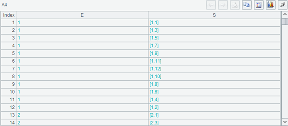
A2 records are repeated in E field. Each A3 record is associated with an A2 record, while each A2 record is associated with 12 A3 records. The length of A4 is the same as that of A3.
This association, which uses part of the primary key fields as a foreign key, is also called primary-sub association. The table with fewer primary key fields is called primary table, and the table with more primary key fields is called sub table. A primary-sub association is a one-to-many association, which is the opposite of a foreign key association. From the standpoint of the sub table to look at the primary table, it is a foreign key relationship, while from the standpoint of the primary table to look at the sub table, it is a primary-sub association.
We will also use this join()to handle the primary-sub association, instead of always using switch() and the join()mentioned in the previous section. Sometimes, we’ll do a groups() to the sub table first and then join() with the primary table. For example, for the previous problem:
| A | B | C | |
|---|---|---|---|
| … | … | ||
| 4 | =A3.groups(eid;sum(salary):salary).keys(eid) | ||
| 5 | =join(A2:E;A4:S) | =A5.groups(E.dept;sum(S.salary)) | |
After A4 performs group aggregation, a table sequence with grouping key as the primary key is formed, which has the one-to-one homo dimension relationship with A2.
Theoretically, in foreign key association, we can also perform a groups()to the fact table using the foreign key as a grouping key to form a table that has the homo dimension relationship with the dimension table, but we usually don’t do that, because a fact table often has multiple foreign keys. If we perform a groups() according to a foreign key, other foreign keys can’t be processed. In most cases, the sub table will only have one primary table, so it is no problem to perform a groups() according to the association key and then do a homo dimension association with the primary table.
Of course, in foreign key association, we can also directly perform join()operation just like in primary-sub association, and put together the records of the dimension table and fact table. One dimension table record may be associated with multiple fact table records. In fact, the join() function mentioned in the foreign key section is doing this, but it also does the action of referencing the dimension table field after association, because this combination action is more common. The length of the result table sequence is also the same as that of the fact table (sub table in the concept of primary-sub association), so the function is also named join().
Now we have encountered several join modes: one-to-one, one-to-many and many-to-one. Is there a many-to-many mode?
There is almost no business meaningful many-to-many join in structured data operations. Many-to-many join only exists in theoretical analysis or mathematical operations. There are basically no associations unrelated to the primary key in daily data processing, so we don’t have to pay attention to them.
SPL provides the xjoin() function to handle join of any conditions, and can also realize many-to-many. But we can only give a mathematical example to illustrate it.
xjoin()will calculate the Cartesian set of the sets involved in the association (note that we say set instead of table sequence, because it is too difficult to find reasonable business examples for structured data). The process can filter the Cartesian product under specified conditions.
For the concept of Cartesian set, unfamiliar readers can search on the Internet. Let’s give a simple example to understand it.
| A | B | C | |
|---|---|---|---|
| 1 | [1,2,3] | [HR,R&D,Sales,Marketing,Admin] | [CHN,USA] |
| 2 | =xjoin(A1:a;B1:b) | =xjoin(A1:a;B1:b;C1:c) | =xjoin(A1:a;C1:c) |
It is not difficult to understand the calculation results of A2,B2,C2. Take a member from each set to form a record, and all possible combinations are included, which is Cartesian product. It can also be understood as a multi-layer loop, and each layer loops through a set. In the innermost loop, the loop variables of each layer are collected to form a record. The set of these records is the result table sequence, and its length is the product of the lengths of the sets involved in the calculation.
In fact, all the associations we mentioned earlier can be defined as follows: take a subset that meets a certain condition from the Cartesian product of the data tables participating in the association (all the join operations we have learned can use the condition of “equal association key value”), and SQL defines the join operation in this way. This definition is very simple, but it does not reflect the associated characteristics between data, which is not helpful to simplify syntax or improve performance.
SPL does not adopt this definition, but describes the common association modes separately. You can use different operation methods in different scenarios.
Let’s use xjoin() to realize the generation of permutations previously realized by recursive program:
| A | B | |
|---|---|---|
| 1 | 5 | 3 |
| 2 | =to(A1) | =B1.(“A2:_”/~).concat(“;”) |
| 3 | =xjoin(${B2}).(~.array()).select(~.id().len()==~.len()) | |
A3 will calculate the permutations of all three members from 1,2,3,4,5.
xjoin()first calculates the Cartesian product of three to(5), and then filters out those with duplicate members (id.len()¹len()), and gets a reasonable permutation.
A1 and B1 can be changed to obtain the permutations of other values.
This code looks much simpler than recursion, but the amount of computation is much larger. We can only try it with smaller values.
We spent three chapters on structured data and its operations. These contents have far exceeded the query and calculation ability of SQL, that is, relational database. Only recursive association in the most common operations has been abandoned because of its difficulty and less application.
In other words, having learned these contents and being able to combine them flexibly, you’ll have a stronger ability to handle structured data than professional database programmers who can only use SQL. Combining with Excel and other tabular software to achieve beautiful presentation, you can easily solve almost all the problems of daily data processing.
SPL Programming - Preface
SPL Programming - 10.3 [Association] Merge
SPL Programming - 11.1 [Big data] Big data and cursor
SPL Official Website 👉 https://www.scudata.com
SPL Feedback and Help 👉 https://www.reddit.com/r/esProcSPL
SPL Learning Material 👉 https://c.scudata.com
SPL Source Code and Package 👉 https://github.com/SPLWare/esProc
Discord 👉 https://discord.gg/2bkGwqTj
Youtube 👉 https://www.youtube.com/@esProc_SPL


