Multidimensional analysis (OLAP) usually requires extremely high response efficiency. When the amount of data involved is large, the performance will be very low if aggregating from detailed data. To solve this problem, a pre-aggregation method to speed up query is usually considered, that is, calculate the results to be queried in advance and read the pre-aggregated results directly at the time of use. In this way, a real-time response can be obtained, so as to satisfy the needs of interactive analysis.

However, it would be unrealistic if all possible dimension combinations were pre-aggregated. For example, when we do the full pre-aggregation of 50 dimensions, even if the intermediate CUBE size is only 1KB, the storage space required will be as large as 1MT, corresponding to one million hard disks with a capacity of 1T each. Even if only 20 of these dimensions are pre-aggregated, it still requires 470,000T of space (visit: for details), which is obvious unacceptable. Therefore, the partial pre-aggregation method is generally adopted, that is, aggregate part of the dimensions to balance the storage space and performance requirements.

The difficult position of pre-aggregation scheme

In fact, even if the storage capacity is ignored, pre-aggregation can only meet relatively fixed query requirements that account for a small proportion of multidimensional analysis, and won’t work once it encounters slightly complex and flexible scenarios that exist in large numbers in actual business.

1) Unconventional aggregation: in addition to the common summation and count operations, some unconventional aggregations such as count unique, median and variance, are likely to be omitted and cannot be calculated from other aggregation values. In theory, there are countless kinds of aggregation operations, and it is impossible to pre-aggregate them all.

2) Aggregation combinations: the aggregation operations may be combined. For example, we may want to know the average monthly sales, which is calculated by adding up the daily sales of a month and then calculating the average. This operation is not a simply summing and averaging operation, but a combination of two aggregation operations at different dimension levels. Such operations are also unlikely to be pre-aggregated in advance.

3) Conditions on metrics: the metrics may also have conditions during the statistics. For instance, we want to know the total sales of orders with transaction amount greater than 100 dollars. This information cannot be processed during pre-aggregation, because 100 will be a temporarily entered parameter.

4)Time period statistics: time is a special dimension, which can be sliced in either enumerating or a continuous interval manner. The starting and ending points of query interval may be fine-grained (for example, to a certain day), in this case, the fine-grained data must be used for re-counting, rather than using the higher-level pre-aggregation data directly.

Indeed, pre-aggregation can improve the performance of multi-dimensional analysis to a certain extent, but it can only deal with very few scenarios in multi-dimensional analysis, and only partial pre-aggregation works. In this case, its usage scenarios are more limited. Even so, it still faces the problem of huge storage space. Therefore, it is unreliable to place hope on the pre-aggregation scheme when pursuing the effect of multidimensional analysis. To make the multidimensional analysis effective, the hard traversal is the basic skill. Even if the pre-aggregated data is available, it can play a greater role only with the aid of excellent hard traversal capability.

Pre-aggregation in SPL

The open-source esProc SPL provides not only the conventional pre-aggregation way in multi-dimensional analysis, but also the special time period pre-aggregation mechanism. More importantly, with the help of SPL's excellent data traversal capabilities, a wider range of scenarios requirements in multi-dimensional analysis can be satisfied.

Let's first look at SPL's pre-aggregation capabilities.

Partial pre-aggregation

Since full pre-aggregation is unrealistic, we can only turn our attention to partial pre-aggregation. Although the response speed of O(1) cannot be achieved, the performance can be improved dozens of times, which is also meaningful. SPL can create multiple pre-aggregated cubes as required. For example, the data table T has five dimensions A, B, C, D and E. According to business experience, we can pre-calculate several most commonly used cubes:

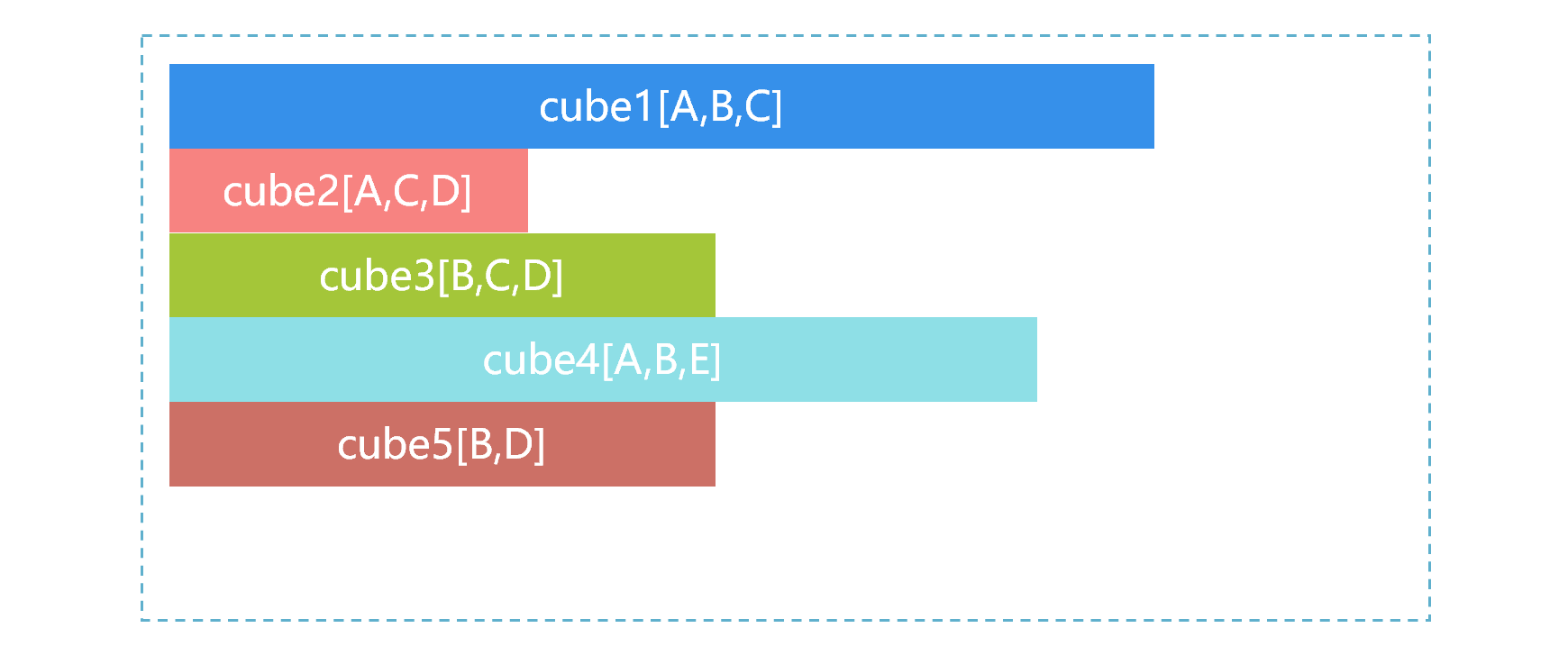
In the figure above, the size of the storage space occupied by the cube is represented by the length of the bar, cube1 is the largest, and cube2 is the smallest. When the front-end application sends a request for aggregation that needs to be made according to B and C, SPL will automatically select from multiple cubes, and the process is roughly as shown below:

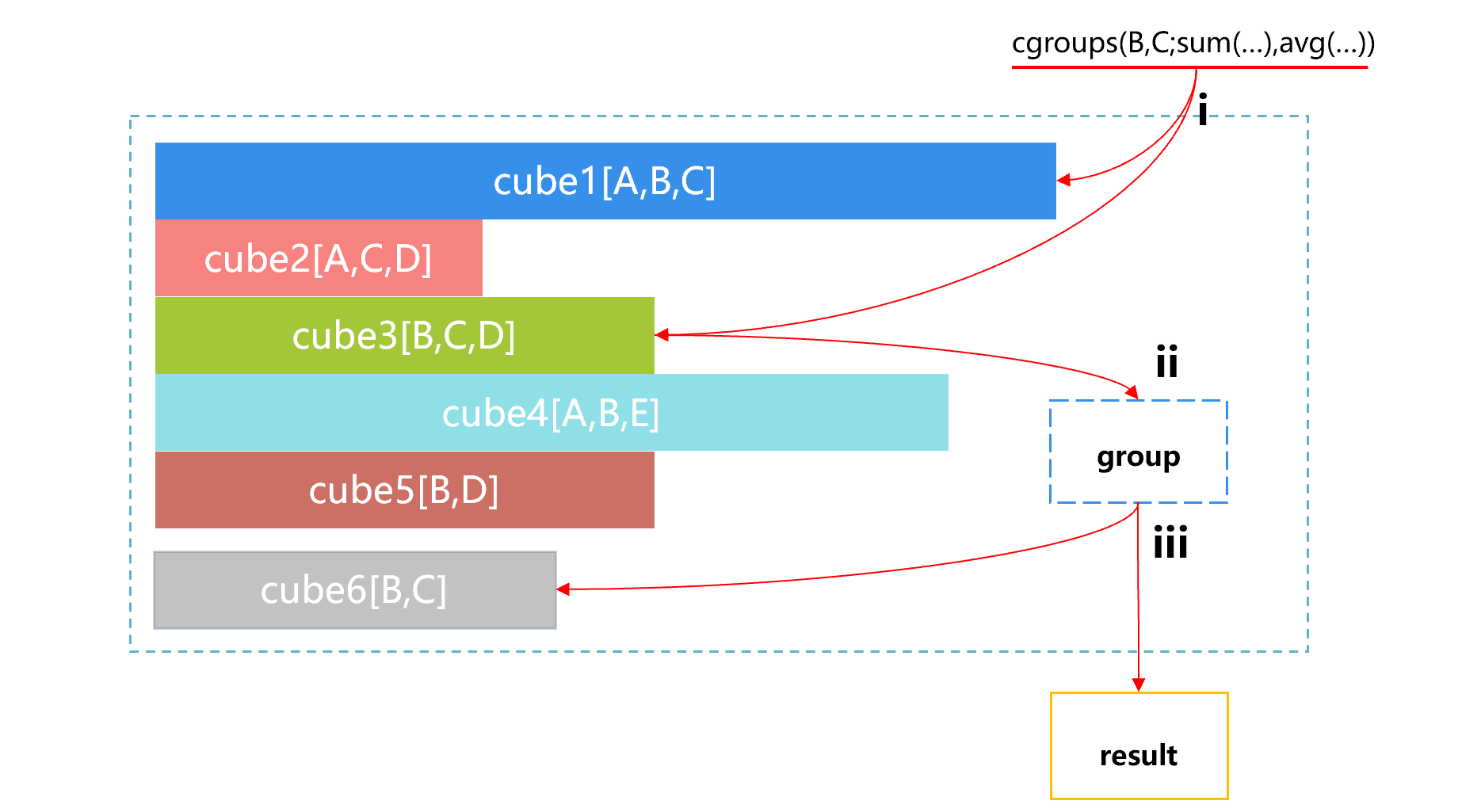
Step i, SPL will find the available cubes, which are cube1 and cube3. Step ii, when SPL finds that cube1 is relatively large, it will automatically select the smaller cube3, and do the grouping and aggregating by B and C based on cube3.

SPL code example:

	A
1	=file("T.ctx").open()
2	=A1.cuboid(cube1,A,B,C;sum(…),avg(…),…)
3	=A1.cuboid(cube2,A,C,D;sum(…),avg(…),…)
4	=A1.cgroups(B,C;sum(…), avg(…))

Using the cuboid function can create the pre-aggregated data (A2 and A3), you need to give a name (such as cube1), and the remaining parameters are the dimension and aggregated metric; when they are used in A4, the cgroups function will automatically use the intermediate cube and select the one with the smallest amount of data according to the above rules.

Time period pre-aggregation

Time is a particularly important dimension in multidimensional analysis, which can be sliced in either enumerating or a continuous interval manner. For example, we need to query the total sales between May 8th and June 12th, the two time points are also passed in as the parameter during the query, which is of highly arbitrary. The counting by time period may also involve multiple association combinations, such as querying the total sales of goods that are sold between May 8th and June 12th and produced between January 9th and February 17th. Such time period counting have strong business significance, but cannot be dealt with using conventional pre-aggregation scheme.

For the special time period counting, SPL provides the time period pre-aggregation way. For example, for the order table, there is already one cube (cube1) pre-aggregated by order date, then we can add one cube (cube2) pre-aggregated by month: In this case, when we want to calculate the total amount from January 22 to September 8, 2018, the approximate process will be:

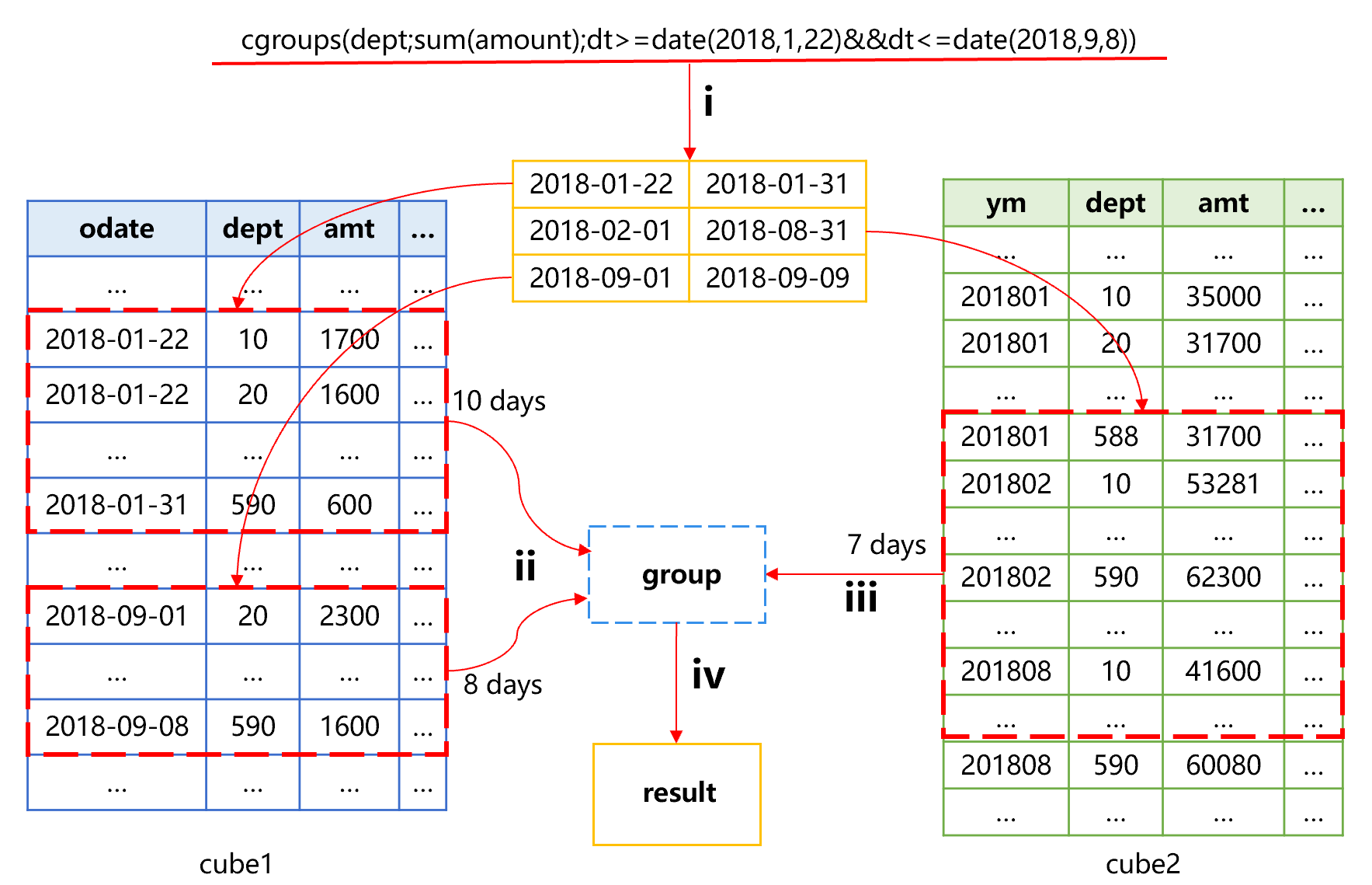
First, divide the time period into three segments, and then calculate the aggregation value of the whole month data from February to August based on the monthly aggregated data cube2, and finally use cube1 to calculate the aggregation values from January 22 to 31 and from September 1 to 8. In this way, the amount of calculation involved will be 7 (Feb. – Aug.) +10 (Jan. 22 - 31) +8 (Sep. 1 – 8) =25; however, if the data of cube1 is used to aggregate, the amount of calculation will be 223 (the number of days from Jan. 22 to Sep. 8). As a result, the calculation amount is reduced almost by 10 times.

SPL code example:

	A
1	=file("orders.ctx").open()
2	=A1.cuboid(cube1,odate,dept;sum(amt))
3	=A1.cuboid(cube2,month@y(odate),dept;sum(amt))
4	=A1.cgroups(dept;sum(amt);odate>=date(2018,1,22)&&dt<=date(2018,9,8))

The cgroups function adds the condition parameter. When SPL finds there are time period condition and higher-level pre-aggregated data, it will use this mechanism to reduce the amount of calculation. In this example, SPL will read the corresponding data from cube1 and cube2 respectively before aggregation.

Hard traversal in SPL

The scenarios that pre-aggregation can cope with are still very limited. To achieve flexible multidimensional analysis, we still need to rely on excellent traversal capability. The multidimensional analysis operation itself is not complicated, and the traversal calculation is mainly to filter the dimension. Traditional database can only use WHERE to perform hard calculation, and treats the dimension-related filtering as a conventional operation, so it cannot obtain better performance. SPL provides a variety of dimension filtering mechanisms, which can meet the performance requirements of various multidimensional analysis scenarios.

Boolean dimension sequence

The most common slicing (dicing) in multidimensional analysis is performed for enumerated type dimension. In addition to time dimension, almost all dimensions are the enumerated dimension such as product, region, type, etc. If the conventional processing method is adopted, the expression in SQL is like this:

SELECT D1,…,SUM(M1),COUNT(ID)… FROM T GROUP BY D1,…

WHERE Di in (di1,di2…) …

where, Di in (di1, di2) is to filter the field values in an enumeration range. In practice, “slicing by customer gender, employee department, product type, etc.” is the slicing of enumerated dimension. For the conventional IN method, only performing multiple comparisons and judgments can the data (slice) that meet the condition be filtered out, and hence the performance is very low. The more values of IN, the worse the performance.

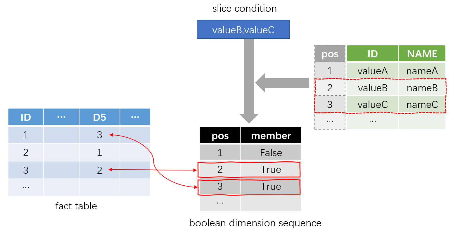
SPL improves the performance by converting the search operation to value accessing operation. First, SPL converts the enumerated dimension to integers. As shown in the figure below, the values of dimension D5 in the fact table are converted to the sequence number (position) in the dimension table:

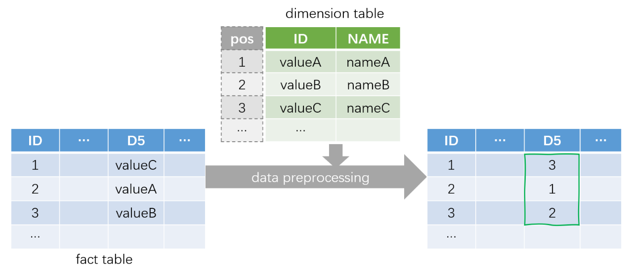
Then, convert the slice condition to an aligned sequence composed of boolean values during query. In this way, the judgment result (true/false) for the value can be taken directly from the specified position of the sequence during comparison to quickly perform the slicing operation.

SPL code example for data preprocessing:

	A
1	=file("T.ctx").open()
2	=file("T_new.ctx”).create(…)
3	=DV=T(“DV.btx”)
4	=A1.cursor().run(D=DV.pos@b(D))
5	=A2.append@i(A4)

A3 reads the dimension table, and A4 uses DV to convert the dimension D to integer. DV will be saved separately for use during query.

Slice aggregation:

	A
1	=file("T.ctx").open()
2	=DV.(V.pos(~))
3	=A1.cursor(…;A2(D))
4	=A3.groups(…)

A2 converts the parameter V to a boolean sequence having the same length as DV. When a member of DV is in V, the member at the corresponding position in A2 will be non-null (playing the role of true when judging), otherwise it will be filled in as null (i.e., false). Then, when traversing to perform slicing, just use the dimension D that has been converted to integer as the sequence number to take the member of this boolean sequence. If it is non-null, it indicates that the original dimension D belongs to the slice condition list V. The operation complexity of taking the value by sequence number is far less than that of IN comparison, which greatly improves the slicing performance.

The excellent hard traversal capability of SPL has obvious application effect in practice. For example, in the case: , with the help of hard traversal technologies such as boolean dimension sequence and pre-cursor filtering, the efficiency for calculating the intersection of bank user profiles and customer groups has been improved by more than 200 times.

Tag bit dimension

In multidimensional analysis, there is also a special enumerated dimension that is often used for slicing (rarely used for grouping and aggregating), and it has only two values, yes/no or true/false. Such enumerated dimension is called the tag dimension or binary dimension, for example, whether a person is married, has attended a college, has a credit card, etc. The slicing of tag dimension belongs to the yes/or type calculation in the filter condition, and when expressed in SQL, it is probably like:

SELECT D1,…,SUM(M1),COUNT(ID)… FROM T GROUP BY D1,…

WHERE Dj=true and Dk=false …

The tag dimension is very common, and tagging the customers or things is an important means in current data analysis. The data set in modern multidimensional analysis often has hundreds of tag dimensions. If such large numbers of dimensions are handled as the ordinary field, it will cause a lot of waste whether in storage or operation, and it will be difficult to obtain high performance.

There are only two values for the tag dimension, only one bit is required to store them. Since a 16-bit integer can store 16 tags, one field is enough for storing these tags that originally require 16 fields. This kind of storage method is called the tag bit dimension. SPL provides this mechanism, which will greatly reduce the storage amount, i.e., the reading amount of hard disk. Moreover, the integer will not affect the reading speed.

For example, we assume there are 8 binary dimensions in total, which are represented by the integer field c1 that stores 8-bit binary numbers. To use the bitwise storage method to calculate the binary dimension slice, the fact table needs to be preprocessed to bitwise storage.

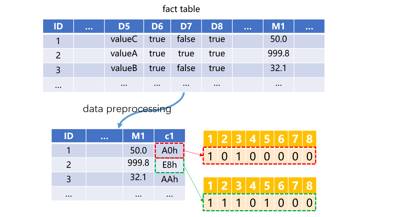
In the processed fact table, the first row c1 is AFh, and is 10100000 after being converted to a binary number, indicating that D6 and D8 are true, and other binary dimensions are false. After that, we can perform bitwise calculation to implement binary dimension slicing.

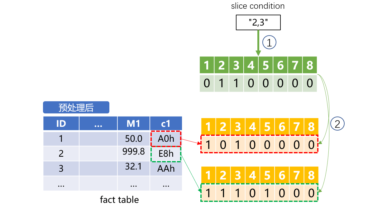
When the slice condition passed in from the front end is "2,3", it means to filter out the data whose values of the second binary dimension (D7) and the third binary dimension (D8) are true, and values of other binary dimensions are false.

SPL code example:

	A	B
1	="2,3"	=A1.split@p(",")
2	=to(8).(0)	=B1.(A2(8-~+1)=1)
3	=bits(A2)
4	=file("T.ctx").open().cursor(;and(c1,A3)==A3)
5	=A4.groups(~.D1,~.D2,~.D3,~.D4;sum(~.M1):S,count(ID):C)

For the 8 yes/or type conditional filtering, it can be achieved by just doing one bitwise AND calculation. In this way, the multiple comparison calculations that need to be performed originally on the binary dimension are converted to one bitwise AND calculation, so the performance is significantly improved. Converting multiple yes/or type values to an integer can also reduce the storage space occupied by the data.

Redundant sorting

Redundant sorting is an optimization method that uses ordered characteristics to speed up reading (traversal) speed. Specifically, store one copy after sorting by dimensions D1,...,Dn, and store another copy after sorting by Dn,...,D1. In this way, although the amount of data will be doubled, it is acceptable. For any dimension D, there will always be a data set that makes D in the first half of its sorted dimension list. If it is not the first dimension, the data after slicing will generally not be concatenated as a single area, but the data are also composed of some relatively large continuous areas. The closer to the top the position of dimension in the sorted dimension list, the higher the degree of physical order of data after slicing will be.

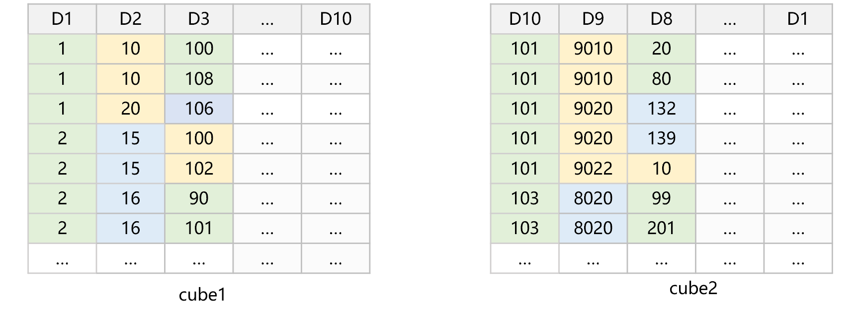
While calculating, it is enough to use one dimension's slicing condition to filter, and the conditions on other dimensions are still calculated during traversal. In multidimensional analysis, the slice on a certain dimension can often reduce the amount of data involved by several times or tens of times. It will be of little significance to reuse the slicing condition on other dimensions. When multiple dimensions have slicing conditions, SPL will choose the dimension whose proportion of after-slice range in the total value range is smaller, which usually means that the amount of filtered data is smaller.

The cgroups function of SPL implements this choice. If there are multiple pre-aggregated data sorted by different dimensions and there are multiple slicing conditions, the most appropriate pre-aggregated data will be chosen.

	A
1	=file("T.ctx").open()
2	=A1.cuboid(cube1,D1,D2,…,D10;sum(…))
3	=A1.cuboid(cube2,D10,D9,…,D1;sum(…))
4	=A1.cgroups(D2;sum(…);D6>=230 && D6<=910 && D8>=100 && D8<=10 &&…)

When cuboid creates the pre-aggregated data, the order of grouped dimensions is meaningful as different pre-aggregated data will be created for different dimension orders. It is also possible to manually choose a properly sorted data set with code, and store more sorted data sets.

In addition, SPL also provides many efficient operation mechanisms, which are not only suitable for multidimensional analysis, but also for other data processing scenarios such as high-performance storage, ordered computing, parallel computing, etc. Combined with these mechanisms, a more efficient data processing experience can be obtained.

As mentioned above, pre-aggregation can only meet relatively simple and fixed requirements that account for a small proportion of multidimensional analysis. For the large number of other common requirements, we still need to use a computing engine (such as SPL) to implement efficient hard traversal to meet. On the basis of excellent hard traversal capability, combined with the partial pre-aggregation and time period pre-aggregation capabilities provided in SPL, we can better meet the performance and flexibility requirements in multidimensional analysis, while minimizing storage cost.

Using SPL to cope with multidimensional analysis scenarios has the advantages of wide coverage, high query performance and low cost, which is the ideal technical solution.