"Principal component analysis is a commonly used dimensionality reduction method, which can trans .."

Lina RaqForum 43 No.
271 View • 1 Years ago

PCA

Principal component analysis is a commonly used dimensionality reduction method, which can transform many highly correlated features into a few features that are independent or unrelated to each other.

For example, the data with 6 samples, 4 features

	x1	x2	x3	x4
1	7	26	6	60
2	1	29	15	52
3	11	56	8	20
4	11	31	8	47
5	7	52	6	33
6	11	55	9	22

Perform dimension reduction on x1,x2,x3,x4

	A
1	[[7,26,6,60],[1,29,15,52],[11,56,8,20],[11,31,8,47],[7,52,6,33],[11,55,9,22],[3,71,17,6],[1,31,22,44],[2,54,18,22],[21,47,4,26],[1,40,23,34],[11,66,9,12],[10,68,8,12]]
2	=pca(A1)
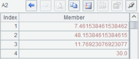
3	=A2(2).((~)/sum(A2(2)))
4	=A3.(cum(~))
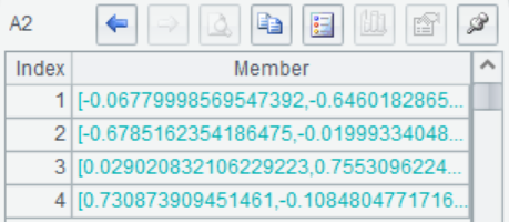
5	=pca@r(A1,2)

A1 The rows of the matrix correspond to the samples and the columns correspond to the features

A2 PCA is performed on A1, return information for dimension reduction

A2(1) Returns the average of each column

A2(2) The principal component variance, which is the eigenvalue corresponding to each eigenvector, is arranged from largest to smallest.

A1(3) Return to the principal component coefficient which is the eigenvector matrix of the covariance matrix

A3 The information contribution rate of four eigenvalues

A4 Calculate the cumulative contribution rate, it can be seen that the sum of the first two features has reached more than 97%, so the first two principal components can be taken.