SQL is wasting lives of data scientists

SQL is difficult to write

Nearly all data scientists use SQL for data exploration and analysis. SQL appears deceptively simple and offers a certain degree of interactivity, making it a seemingly ideal choice for these purposes.

To perform filtering and grouping operations, for example, SQL just needs one line of code:

select id,name from T where id=1
select area,sum(amount) from T group by area

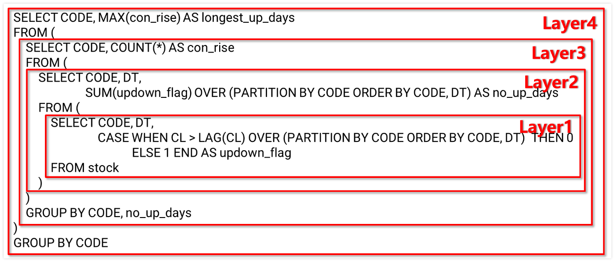
But this is only limited to simple cases. When the computation becomes complex, SQL code becomes complicated, too. For example, to count the longest consecutive rising days of each stock, the SQL statement is as follows:

SELECT CODE, MAX(con_rise) AS longest_up_days
FROM (
    SELECT CODE, COUNT(*) AS con_rise
    FROM (
        SELECT CODE, DT, SUM(updown_flag) OVER (PARTITION BY CODE ORDER BY CODE, DT) AS no_up_days
        FROM (
            SELECT CODE, DT, 
                CASE WHEN CL > LAG(CL) OVER (PARTITION BY CODE ORDER BY CODE, DT)  THEN 0
                ELSE 1 END AS updown_flag
            FROM stock
        )
    )
    GROUP BY CODE, no_up_days
)
GROUP BY CODE

And to perform the commonly seen funnel analysis on user behavior data in e-commerce industries:

WITH e1 AS (
	SELECT uid,1 AS step1, MIN(etime) AS t1
	FROM events
	WHERE etime>=end_date-14 AND etime<end_date AND etype='etype1'
	GROUP BY uid),
e2 AS (
	SELECT uid,1 AS step2, MIN(e1.t1) as t1, MIN(e2.etime) AS t2
	FROM events AS e2 JOIN e1 ON e2.uid = e1.uid
	WHERE e2.etime>=end_date-14 AND e2.etime<end_date AND e2.etime>t1 AND e2.etime<t1+7 AND etype='etype2'
	GROUP BY uid),
e3 as (
	SELECT uid,1 AS step3, MIN(e2.t1) as t1, MIN(e3.etime) AS t3
	FROM events AS e3 JOIN e2 ON e3.uid = e2.uid
	WHERE e3.etime>=end_date-14 AND e3.etime<end_date AND e3.etime>t2 AND e3.etime<t1+7 AND etype='etype3'
	GROUP BY uid)
SELECT SUM(step1) AS step1, SUM(step2) AS step2, SUM(step3) AS step3
FROM e1 LEFT JOIN e2 ON e1.uid = e2.uid LEFT JOIN e3 ON e2.uid = e3.uid

Both examples involve multilayer nested subqueries, which are difficult to understand and more difficult to write.

There are many similar computing tasks in real-world business scenarios. For example:

• Find players who score three times continuously in one minute;

• Find the number of users in 7 days who are active in three continuous days;

• Compute retention rate of every day’s new users a business retains in the next day;

• Compute the growth rate of a stock on the date when the price is both greater than both the previous and the next five days;

• …

These complex requirements often necessitate multi-step procedures and involve order-based operations. Their SQL implementations are extremely roundabout with a nearly one hundred lines of N-layered nested statement. Data scientists are wasting their lives in writing such SQL statements.

SQL is difficult to debug

Complicated SQL statements are very inconvenient to debug, such as the above commonly seen complex nested SQL statements. To debug them, we need to disassemble the statement and perform debugging layer by layer. Thedisassembly process involves modification of the SQL statement, making the whole debugging procedure very complicated.

This is because SQL does not have common debugging methods such as “set breakpoint” and “step over”. And data scientists have to go to the trouble of disassembling statements in order to perform debugging, which is a waste of their lives.

SQL has low performance

The query performance of SQL heavily depends on database optimizer. A well-designed database product is able to automatically adopt a more efficient algorithm (instead of executing the SQL statement literally), but often the optimization mechanism breaks down when facing complex computing logics.

Here is a simple example. To fetch the top 10 from 100 million records, SQL has the following code:

SELECT TOP 10 x FROM T ORDER BY x DESC

Though this SQL statement contains the ORDER BY keyword, database optimizer will use a more efficient algorithm instead of performing the full sorting (because big data sorting is very slow).

Now let’s modify the task to find the top 10 from each group, and SQL has the following implementation:

SELECT * FROM (
 SELECT *, ROW_NUMBER() OVER (PARTITION BY Area ORDER BY Amount DESC) rn
 FROM Orders )
WHERE rn<=10

The implementation only gets a little complicated, but most database optimizers already become incapable of performing the optimization. They cannot guess the SQL statement’s purpose but can only execute the literal logic written in the statement to perform the sorting (as there is ORDER BY keyword). As a result, performance is sharply decreased.

The SQL statements in real-world business scenarios are far more complicated than that in the example. It is rather common that database optimizer becomes ineffective, such as the above SQL statement handling funnel analysis. The statement involves repeated joins, which are difficult to write and extremely slow to execute.

Low performance means waiting. For certain big data processing cases, waiting times are from a number of hours to even one day. And during the long waits data scientists’ lives passed.

SQL is closed

SQL is the formal language used by databases. The closed databases make data processing difficult. Being closed here refers to the database requirement that data to be computed and processed by the database should be loaded into it in advance. The border between internal data and external data is clear.

In real-life businesses, data analysts often need to process data coming from the other sources, including text, Excel, application interface, web crawler, to name a few. Sometimes data coming from any of those sources is only temporarily used, but loading them into the database for each use consumes database space resources and the ETL process is time-consuming. And databases usually have constraints, and non-standardized data cannot be loaded into. This requires to first re-organize data, which needs both time and resources, and then write them to the database, which is also time-consuming (as database writes are very slow). It is during handling these peripheral data organization, loading and retrieval operations that the life of a data scientist is wasted.

Python is also wasting lives of data scientists

As SQL has too many problems, data scientists seek its replacements, and Python is one of them.

Python surpasses SQL in many aspects. It is easier to debug and more open, and supports procedural computation. However, Python also has its flaws.

Complex computations are still hard to handle

Pandas, one of Python’s third-party libraries, offers a rich collection of computing functions, which make certain computations simpler than their SQL counterparts. However, handling complex scenarios may still be challenging. For example, here is the code for finding the longest consecutive rising days for each stock mentioned earlier:

import pandas as pd
stock_file = "StockRecords.txt"
stock_info = pd.read_csv(stock_file,sep="\t")
stock_info.sort_values(by=['CODE','DT'],inplace=True)
stock_group = stock_info.groupby(by='CODE')
stock_info['label'] = stock_info.groupby('CODE')['CL'].diff().fillna(0).le(0).astype(int).cumsum()
max_increase_days = {}
for code, group in stock_info.groupby('CODE'):
	max_increase_days[code] = group.groupby('label').size().max() – 1
max_rise_df = pd.DataFrame(list(max_increase_days.items()), columns=['CODE', 'max_increase_days'])

The Python code, which involves hard-coding with “for” loop, is still cumbersome. This continues to waste lives of data scientists.

Inconvenient debugging functionalities

Python has many IDEs and provides much-better-than-SQL debugging capabilities such as “breakpoint”, which makes it unnecessary to disassemble the code.

But viewing intermediate values still mainly relies on the print method, which needs to be removed after debugging. This proves to be somewhat cumbersome.

It takes longer to debug when the corresponding functionality is inconvenient to use, which results in a waste of time for data scientists.

Low big data processing capability and performance

Python almost does not have any big data processing capabilities. While the Pandas library can perform in-memory computations like sorting and filtering directly, it struggles with datasets larger than the available memory. In that case data needs to be segmented and processed segment by segment with hardcoding, and the code becomes very complicated.

Python's parallelism is superficial. To harness multiple CPUs, complex multi-process parallelism is often required. But this is beyond the reach of most data scientists. Bing unable to code parallel processing, data scientists can only perform the slow serial computations and witness their time wasted.

Both SQL and Python are not satisfactory enough, then what can truly rescue data scientists?

esProc SPL – the rescuer of data scientists

esProc SPL! A very tool specifically designed for structured data processing.

SPL is characterized by conciseness, ease of understanding and convenient debugging. It supports large-scale data processing and delivers high performance, fundamentally addressing limitations of SQL and Python.

Simple to write

SPL offers rich data types and computing class libraries and supports procedural computation, greatly simplifying the code of implementing complex computations. To find the longest consecutive rising days for each stock, for example, SPL has the following code:

	A
1	=stock.sort(StockRecords.txt)
2	=T(A1).sort(DT)
3	=A2.group(CODE;~.group@i(CL<CL[-1]).max(~.len()):max_increase_days)

The SPL code is much shorter and does not involve the loop statement. Both data read and write are not difficult.

To perform the ecommerce funnel analysis:

	A
1	=["etype1","etype2","etype3"]
2	=file("event.ctx").open()
3	=A2.cursor(id,etime,etype;etime>=end_date-14 && etime<end_date && A1.contain(etype) )
4	=A3.group(uid)
5	=A4.(~.sort(etime)).new(~.select@1(etype==A1(1)):first,~:all).select(first)
6	=A5.(A1.(t=if(#==1,t1=first.etime,if(t,all.select@1(etype==A1.~ && etime>t && etime<t1+7).etime, null))))
7	=A6.groups(;count(~(1)):step1,count(~(2)):step2,count(~(3)):step3)

Compared with its SQL counterpart, the SPL code is more concise and versatile, and more conforms to the natural way of thinking. It can be used to handle the funnel analysis involving any number of steps. E-commerce funnel analysis with SPL is simpler and aligns more with natural thinking. This code can handle any-step funnel, offering greater simplicity and versatility compared to SQL.

Convenient to debug

SPL also offers comprehensive debugging capabilities, including “Set breakpoint”, “Run to cursor”, “Step over”, etc. The result of each step is displayed in real-time on the right side of the IDE. This is convenient as users do not need to split away each subquery or perform manual print any more.

Support for big data processing

SPL supports big data processing, no matter whether the data can fit into the memory or not.

In-memory computation:

	A
1	=d:\smallData.txt
2	=file(A1).import@t()
3	=A2.groups(state;sum(amount):amount)

External memory computation:

	A
1	=d:\bigData.txt
2	=file(A1).cursor@t()
3	=A2.groups(state;sum(amount):amount)

We can see that the SPL code for the external memory computation is the same as that for the in-memory computation, requiring no additional workload.

It is easy and convenient to implement parallel processing in SPL. You just need to add an @m option to the serial computation code.

	A
1	=d:\bigData.txt
2	=file(A1).cursor@tm()
3	=A2.groups(state;sum(amount):amount)

High performance

It is easy to write code with low amount of computational work and achieves faster execution in SPL. Take the previously mentioned topN problem as an example, SPL treats topN as a kind of aggregation, eliminating full sorting from the computing logic and achieving much faster speed. This SPL capability is inherent and does not rely on the assistance of optimizer.

Get TopN from the whole set:

Orders.groups(;top(10;-Amount))

Get TopN from each group:

 Orders.groups(Area;top(10;-Amount))

The code of getting topN from each group and that from the entire set is basically the same. Both are straightforward and runs fast.

SPL offers a wide range of high-performance algorithms, including:

• For search: Binary search, sequence-number-based location, index-based search, batch search, etc.

• For traversal: Cursor filtering, multipurpose traversal, multicursor, new understanding of aggregation, order-based grouping, application cursor, column-wise computing, etc.

• For association: Foreign-key-based pre-association, foreign key numberization, alignment sequence, big dimension table search, one-sided heaping, order-based merge, association-based location, etc.

• For cluster computing: cluster composite table, duplicate dimension table, dimension table segmentation, load balancing, etc.

Equipped with these algorithms, SPL can achieve a dramatic skyrocketing in computational performance. Data scientists do not need to waste their lives in long waiting.

Open system

SPL is naturally open. It can directly compute any data sources as long as it can access them, including data files such as CSV and Excel, various relational and non-relational databases, and multi-layer data such as JSON and XML, and thus can perform mixed computations.

With the open system, data scientists can process data coming from various sources directly and efficiently, getting rid of the time spent in data organization and data import/export and thus increasing data processing efficiency.

High portability and enterprise-friendly

SPL also offers the proprietary file format that is high-performance and portable.

	A
1	=d:\bigData.btx
2	=file(A1).cursor@t()
3	=A2.groups(state;sum(amount):amount)

In contrast, Python lacks a proprietary storage solution. Text files are slow, and databases result in the loss of portability.

SPL is enterprise-friendly because it is developed in pure Java. After data exploration and analysis, data scientists can integrate SPL with the application by embedding its jars into the latter, facilitating smooth transition from outside to inside.

With the convenient to use, easy to debug, high-performance and integration-friendly SPL, data scientists can be freed from the heavy coding work and devote more time to their own businesses.