Background

Often a report has diverse data sources, which can be RDB, NoSQL, text, Excel and MQ.

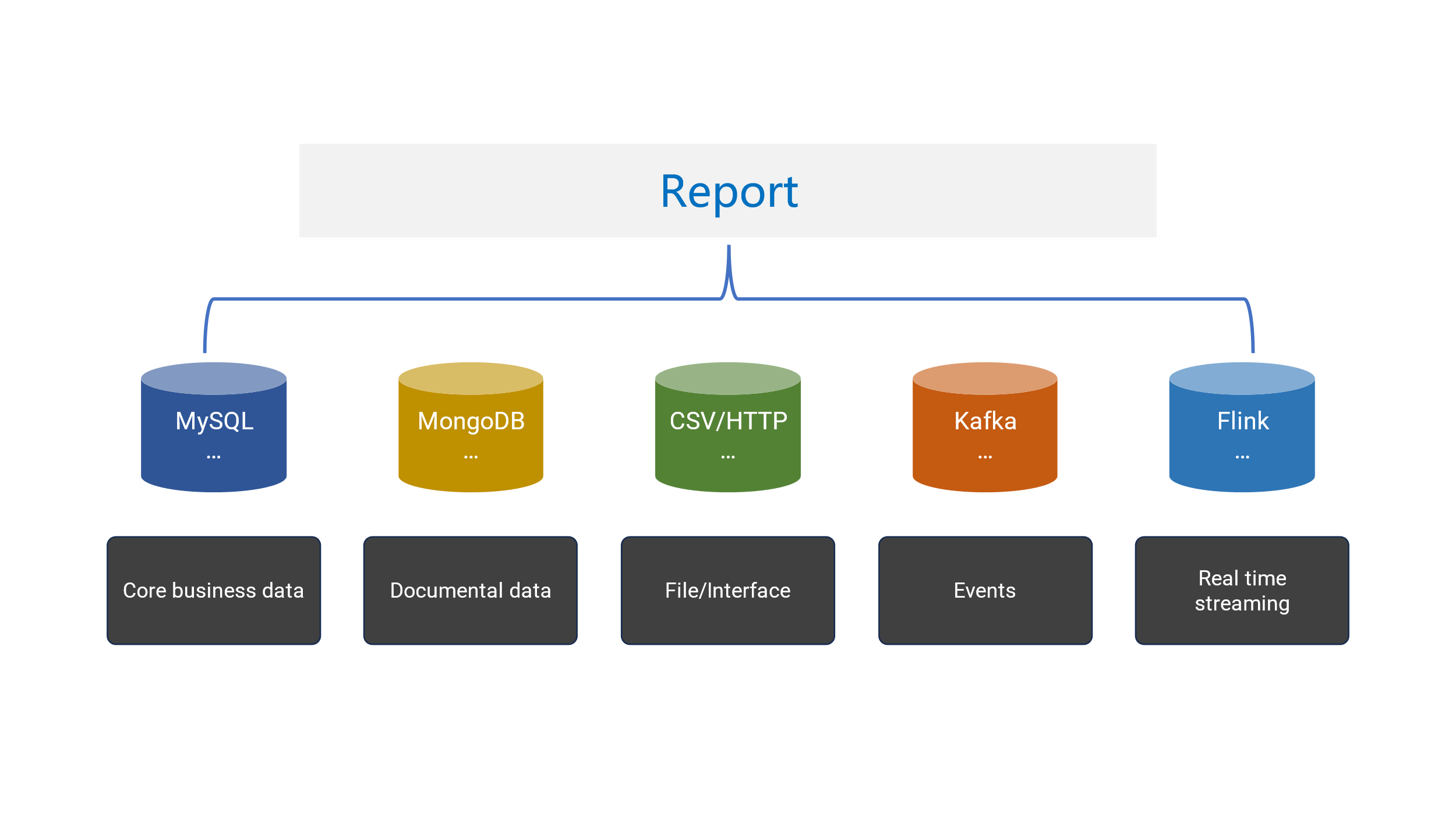
Logical data warehouses can facilitate mixed-source computations to some extent. But logical data warehouse frameworks are too heavy and complex, and cumbersome pre-processing is needed for operations, maintenance and management, making them more suitable for creating platform solutions for large-scale organizations. This is too heavy for an ordinal report. The cost of specifically building a logical data warehouse is not worth the gain.

SPL approach

SPL provides real-time mixed-data source computing capability, enabling mixed-source computations on any accessible data sources. SPL’s this functionality is very lightweight and can be directly embedded into the reporting application to work. Here are relationships between reports, SPL and data sources:

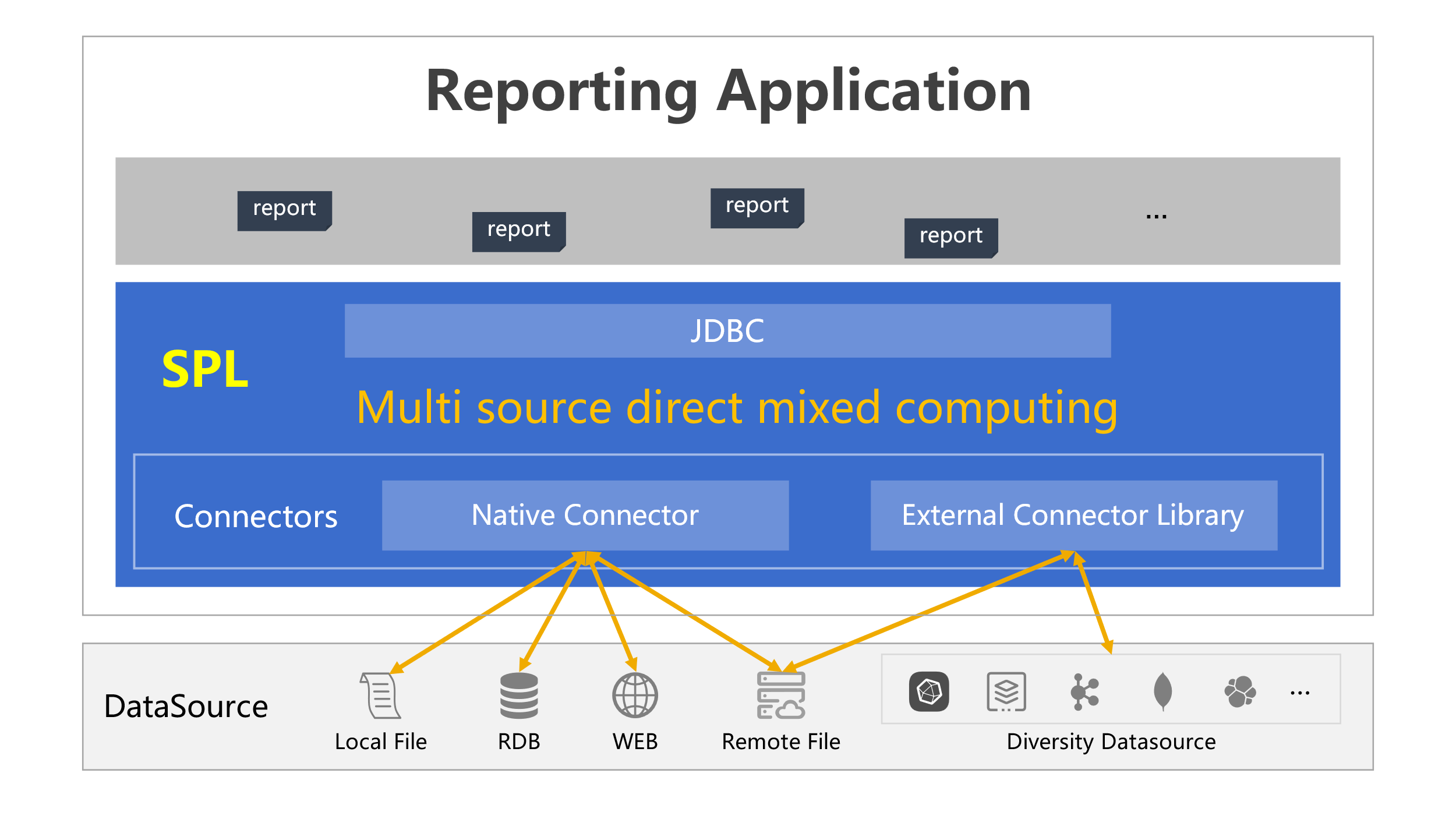
SPL has two types of data source connectors: native connectors and external connectors. Native connectors, which are built in the SPL core system, include the most commonly seen RDBs, local files such as text files, Excel files, JSON file, and HTTP data sources. External connectors encompass various other data sources, such as MongoDB, Kafka, ElasticSearch, and cloud storage, which are not part of the SPL core system and require separate deployment.

Unlike logical data warehouses’ mapping mode, SPL supports and encourages using a data source’s native syntax to access and compute data. If the data source’s computing ability is insufficient, SPL offers supplements, which will be demonstrated in the following examples.

SPL supports a vast variety of data sources. Only some of them, including the most common ones, are listed below:

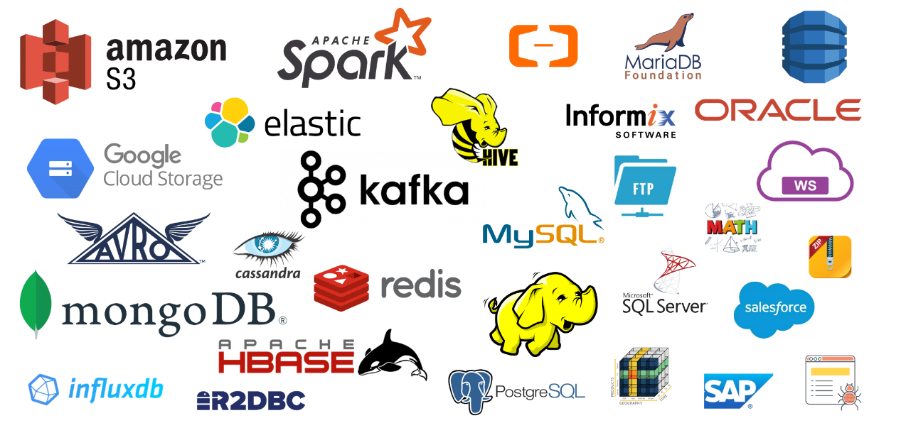
In which the native connectors can connect to JDBC data sources such as MySQL and Oracle, local files such as CSV, Excel and JSON, web data sources like HTTP and REST API, and remote files, etc.

SPL offers two types of data objects – table sequence and cursor, for storing data accessed from sources. They correspond to in-memory data table and streaming data table respectively.

Almost all data sources, including RDBs, provide these two types of data object interfaces, through which smaller datasets are read all at once into in-memory data tables, and large datasets are retrieved incrementally using stream-style cursor. With these two types of data objects, SPL can accommodate nearly all data sources.

Unlike logical data warehouses, SPL does not require pre-defined metadata for mapping. Instead, it accesses data directly using methods provided by the data source and encapsulates data as one of these two types of data objects.

This helps preserve characteristics of the data source and fully leverage its storage and computing capabilities. There is also no need to perform any preliminary data import actions, as it can access data in real-time.

Next, let’s take a look at the specific uses.

Configuring data sources through connector configuration in SPL IDE

Configure the most common JDBC connection for a native connector within the IDE, like MySQL. Then copy database driver jar to [SPL installation directory]/common/jdbc. Now configure the standard MySQL JDBC connection, as shown below:

Download the corresponding external library driver package (Download) for an external connector, decompress it to any directory ([SPL installation directory]\esProc\extlib by default), and load the external library.

There are dozens of uncommon data sources and functions in the external library list:

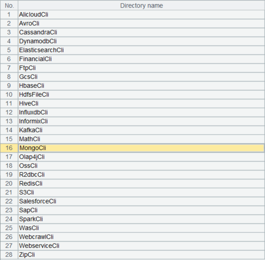
External connectors are located in the external libraries, which serve as the extension libraries provided by SPL for holding specialized functions. These functions, which are not commonly used in general scenarios, can be loaded ad hoc from the external libraries as needed.

There are various types of external data sources, and not all are commonly used. Therefore, offering these connectors as external libraries provides greater flexibility, allowing for the timely addition of new data sources without impacting the existing ones in the future.

Most external libraries are external connectors.

Click on Tool -> Options -> Environment on the IDE menu, and select the external library directory where you just downloaded and decompressed.

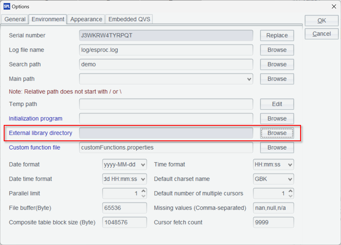
There will be a list of all external libraries. Select the libraries you need to load.

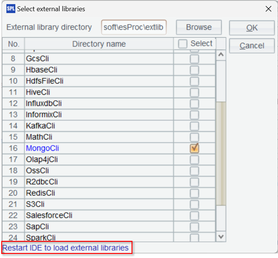
Here MongoDB is checked. Then click “OK” button and restart the IDE to take effect.

Use cases

Mixed MongoDB-MySQL query

Our example originates from the e-commerce business and utilizes MySQL to store orders information. The structures of the two tables involved, orders and order_items, are as follows:

Orders:

Field	Type	Description
order_id	INT (PK)	Order ID
user_id	INT	User ID
order_date	DATETIME	The date when an order is placed
total_amount	DECIMAL(10, 2)	Order amount

Order_items:

Field	Type	Description
order_item_id	INT (PK)	Item ID
order_id	INT（FK）	Order ID
product_id	VARCHAR(20)	Product ID
quantity	INT	Purchase quantity
price	DECIMAL(10, 2)	Unit price

These two tables are associated through order_id.

The product information changes as related types – brand, model and specifications for electronics, and brand, size and color for clothing, change, so MongoDB is used to store it. The “attributes” field accommodates dynamic attributes.

Field	Description
product_id	Product ID (through which data is associated with MySQL)
name	Product name
brand	Brand
category	Category
attributes	Dynamic attribute

The set of products is associated with MySQL via product_id.

These are sample data in MySQL and MongoDB.

Orders:

order_id	user_id	order_date	total_amount
1	101	2024-09-01	1999.99
2	102	2024-09-02	1599.99
…

Order_items:

order_item_id	order_id	product_id	quantity	price
1	1	prod_1001	1	999.99
2	1	prod_1002	1	1000.00
3	2	prod_1003	1	1599.99
…

MongoDB：

{
  "product_id": "prod_1001",
  "name": "Smartphone X",
  "brand": "BrandA",
  "category": "Electronics",
  "attributes": {
    "color": "Black",
    "storage": "128GB"
  }
},
{
  "product_id": "prod_1002",
  "name": "Laptop Y",
  "brand": "BrandB",
  "category": "Computers",
  "attributes": {
    "processor": "Intel i7",
    "ram": "16GB"
  }
…
}

We want to query the total sales of three products – “Tablets”, “Wearables” and “Audio” (product categories) in the past month (period of time). This involves mixed queries on MySQL and MongoDB.

SPL script (orderAmount.splx):

	A
1	=connect("mysql")
2	=A1.query@x("SELECT o.order_id, o.user_id, o.order_date, oi.product_id, oi.quantity, oi.price FROM orders o JOIN order_items oi ON o.order_id = oi.order_id WHERE o.order_date >= CURDATE()- INTERVAL 1 MONTH")
3	=mongo_open("mongodb://127.0.0.1:27017/raqdb")
4	=mongo_shell@d(A3, "{'find':'products', 'filter': { 'category': {'$in': ['Tablets', 'Wearables', 'Audio'] } }}” )
5	=A2.join@i(product_id,A4:product_id,name,brand,category,attributes)
6	=A5.groups(category;sum(price*quantity):amount)
7	return A6

A1 connects to MySQL, then A2 queries the order data in the past month using SQL. @x option enables closing the connection after querying is finished. Below is the query result:

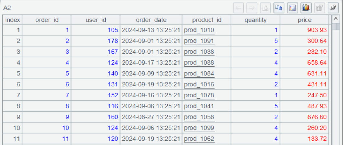
A3 connects to MongoDB.

A4 uses mongo_shell function to query and filter data, where @d option enables returning a table sequence. Function parameters are JSON strings conforming to the MongoDB Command specification, which is the MongoDB native syntax. You can see that the data meeting the criteria is retrieved.

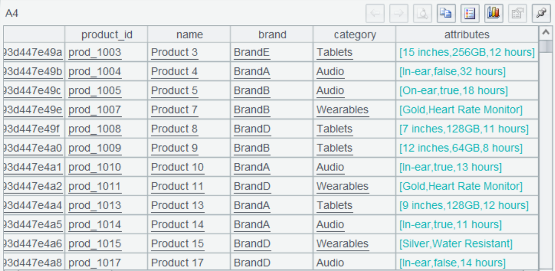
A5 associates the two parts through product_id, and this is the association result:

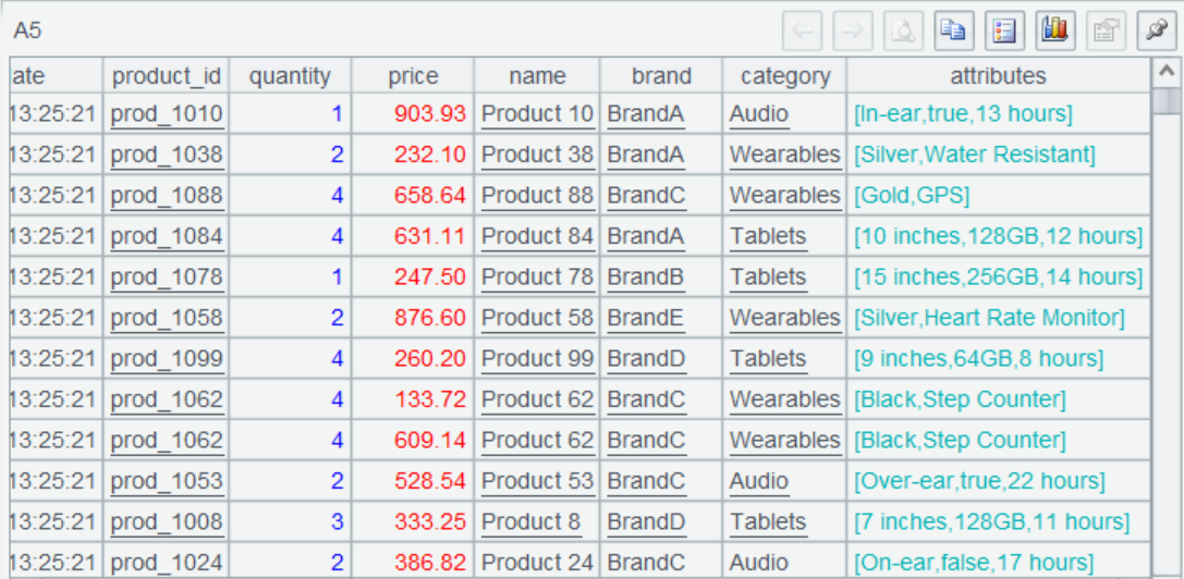
A6 summarizes the order amount by product type to get the final result.

A7 uses return statement to return the final result set to the report.

Mixed Kafka-MongoDB query

We will then use Kafka to illustrate the computation.

Based on the previous scenario, we use Kafka to publish the order and product information. When the user places an order, the order data will be sent to the order subject by the producer.

Let’s first look at the producer script:

	A
1	=kafka_open("/mafia/my.properties","topic-order")
2	[ { "order_id": "1", "user_id": "101", "product_id": "prod_1001", "quantity": 1 }, … ]
3	=kafka_send(A1, "A101", json(A2))
4	=kafka_close(A1)

A1 connects to the Kafka server, and below is the content of the property file my.properties:

bootstrap.servers=localhost:9092
client.id=SPLKafkaClient
session.timeout.ms=30000
request.timeout.ms=30000
enable.auto.commit=true
auto.commit.interval.ms=1000
group.id=spl-consumer-group
key.serializer=org.apache.kafka.common.serialization.StringSerializer
value.serializer=org.apache.kafka.common.serialization.StringSerializer
key.deserializer=org.apache.kafka.common.serialization.StringDeserializer
value.deserializer=org.apache.kafka.common.serialization.StringDeserializer

A2 is the order data to be sent, which is typically received from a transmitting program. We write it directly here.

A3 sends the order data, and A4 closes the connection.

The report’s data source is the consumer script (orderConsumer.splx). To query information of products in a specified category, first we need to set the product category parameter:

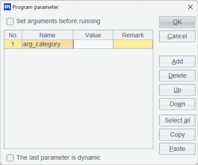
Here is the consumer script:

	A
1	=kafka_open("/mafia/my.properties","topic-order")
2	=kafka_poll(A1)
3	=json(A2.value)
4	=mongo_open("mongodb://127.0.0.1:27017/raqdb")
5	=mongo_shell@d(A4,"{'find':'products'}")
6	=A3.join(product_id,A5:product_id,product_id,name,brand,category,attributes)
7	return A6.select(category== arg_category)

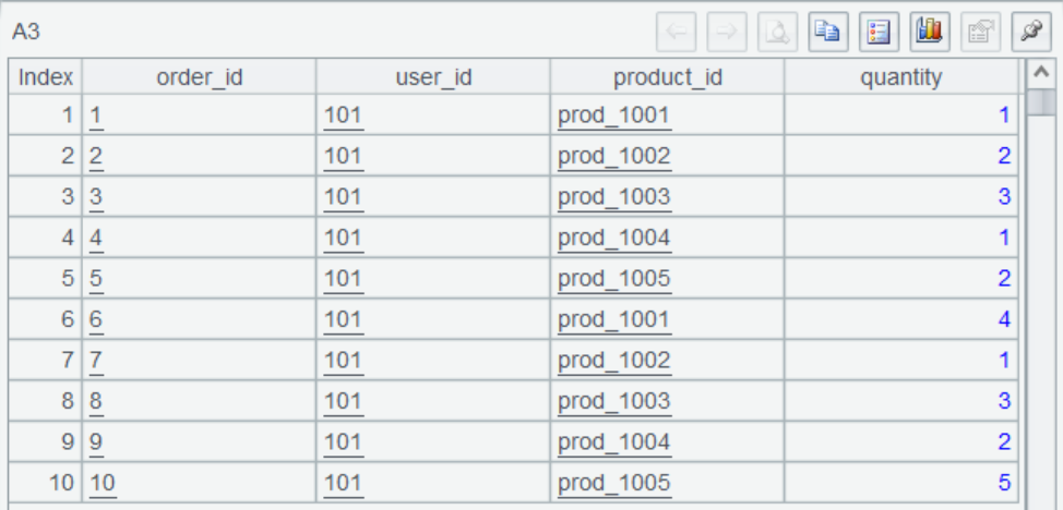
A2 retrieves consumer records and returns a table sequence. The result is as follows:

A3 converts the JSON string order data to a table sequence:

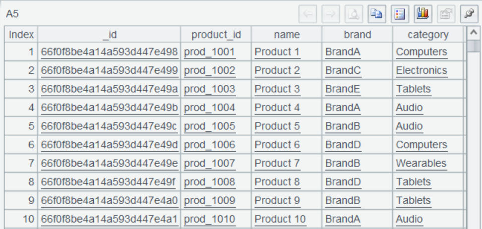
A5 queries product data:

A6 obtains all order and product information based on the association via product_id:

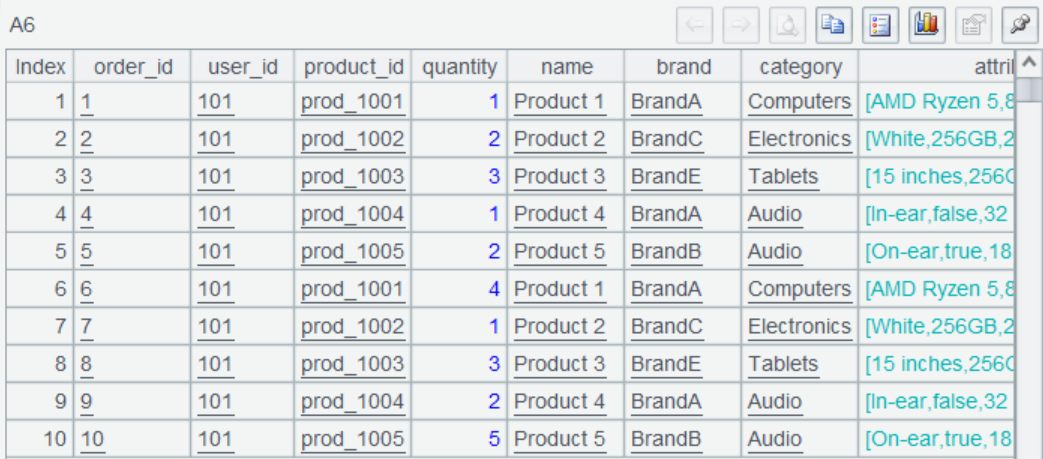
Last, A7 gets the eligible records according to the specified condition and returns query result set to the report. At this point, the association between Kafka and MongoDB is completed.

Big data situation

Sometimes the report query involves large volumes of data, full reading is slow and may lead to memory overflow. To handle such cases, SPL offers cursor mechanism to read data gradually in a streaming fashion.

Let’s modify the previous example of mixed MySQL-MongoDB computation:

	A
1	=connect("mysql")
2	=A1.cursor@x("SELECT o.order_id, o.user_id, o.order_date, oi.product_id, oi.quantity, oi.price FROM orders o JOIN order_items oi ON o.order_id = oi.order_id WHERE o.order_date >= CURDATE() - INTERVAL 1 MONTH ORDER BY oi.product_id ASC")
3	=mongo_open("mongodb://127.0.0.1:27017/raqdb")
4	=mongo_shell@dc(A3,"{'find':'products','filter': {},'sort': {'product_id': 1}}")
5	=joinx(A2:o,product_id;A4:p,product_id)
6	=A5.groups(p.category;sum(o.price*o.quantity):amount)
7	return A6

A2 changes the original “query” to “cursor”, which returns a cursor object without truly fetching the data.

Using @c option in A4 means that the queried MongoDB data also returns as a cursor, and the result is also a cursor object.

A5 uses joinx() function to associate two cursors, which necessitates that both cursors be ordered by the joining fields. For this reason, a sorting operation is performed in both A2’s SQL and the MongoDB command in A4.

The association result of A5 is still a cursor. When fetch() function retrieves data, the actual result is a multi-layer table sequence:

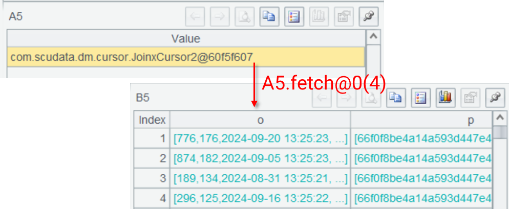
A6 performs aggregation by category and obtains the result. It is only at this point that data is fetched and computed for all cursor operations.

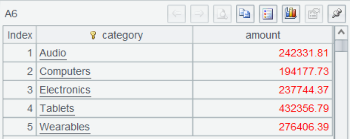
A7 returns the final result to the report. The SPL cursor can be used to handle big data situations involving almost any data sources.

Using SPL within the reporting application

Let’s look at how to use SPL in a reporting application.

Integration with the application

It is simple to integrate SPL with the reporting application. Just need to import SPL’s two jars – esproc-bin-xxxx.jar and icu4j-60.3.jar (generally in [installation directory]\esProc\lib) to the application, and then copy raqsoftConfig.xml (also in [installation directory]\esProc\lib) to the application’s class path.

raqsoftConfig.xml is SPL’s core configuration file, and its name cannot be changed.

Configure the external library in raqsoftConfig.xml as needed. To use MongoDB and Kafka, for example:

<importLibs>
    <lib>KafkaCli</lib>
    <lib>MongoCli</lib>
</importLibs>

At the same time, the MySQL data source also needs to be configured here. Configure the connection information under the DB node:

<DB name="mysql">
    <property name="url" value="jdbc:mysql://127.0.0.1:3306/raqdb?useCursorFetch=true"/>
    <property name="driver" value="com.mysql.cj.jdbc.Driver"/>
    <property name="type" value="10"/>
    <property name="user" value="root"/>
    <property name="password" value="root"/>
    <property name="batchSize" value="0"/>
    <property name="autoConnect" value="false"/>
    <property name="useSchema" value="false"/>
    <property name="addTilde" value="false"/>
    <property name="caseSentence" value="false"/>
</DB>

Access to SPL from reports

SPL encapsulates the standard JDBC interface. Reports can access SPL by configuring data sources in JDBC. The configurations of report data sources are as follows:

<Context>
    <Resource name="jdbc/esproc"
              auth="Container"
              type="javax.sql.DataSource"
              maxTotal="100"
              maxIdle="30"
              maxWaitMillis="10000"
              username=""
              password=" "
              driverClassName=" com.esproc.jdbc.InternalDriver "
              url=" jdbc:esproc:local:// "/>
</Context>

The standard JDBC call is the same as that for an ordinary database, so we will not elaborate further.

Then call the SPL script from the report data set in the way of calling the stored procedure to get SPL’s computing result.

Call the order amount computation script orderAmount.splx:

call orderAmount()

Call the order query script having parameters orderConsumer.splx:

call orderConsumer(?)

In which the question mark ? represents the specified product category parameter. Its value is specified during report query.

In this essay we only illustrate mixed computations on some data sources. Actually, SPL supports a wide variety of data sources, and can extend to include new ones.

By offering consistent data objects, SPL can deal with mixed-computations between any accessible data sources in a very simple way. This enables reports to obtain real-time mixed query ability and helps achieve mixed-source, real-time reports efficiently.