SPL Achieves Window Function Functionality for MySQL
Added only in the SQL2003 standard, SQL window functions are used to deal with certain complicated calculations. The popular MySQL database, however, hadn’t been window-function-friendly until a recent version, which partly supports the functions, was released. Yet the insufficient support of window functions makes it a headache to MySQL users.
Indeed, same functionalities can be realized in MySQL through SQL statement composition. But user-defined variables are needed and the implicit rule that multiple SELECT expressions should be calculated from left to right needs to be observed. Here are two examples (For the convenience of debugging, the test environment is esProc).
1. Sales ranking in January 2016
| A | |
|---|---|
| 1 | set @i1=0, @i2=0, @d1=null; |
| 2 | select @i1:=@i1+1 `row_number`, province, curr_sales, prev_sales, @i2:=if(prev_sales=curr_sales,@i2,@i1) `rank` from (select province, cast(@d1 as decimal(15,2)) as prev_sales, @d1:=sales as curr_sales from detail where yearmonth=201601 order by sales desc ) t1; |
| 3 | =connect("mysql") |
| 4 | >A3.execute(A1) |
| 5 | =A3.query@x(A2) |
(1) A1’s statement initializes user-defined variables;
(2) A2’s statement sorts sales amounts in descending order and then compares each sales amount with the previous one. The rank remains unchanged if the two amounts are equal; otherwise it is changed to the row number;
(3) A3 connects to the database;
(4) A4 executes A1’s initialization statement;
(5) A5 executes A2’s query, closes database connection and returns result.
Below is A5’s result and what we want:
2. Percentile ranks of sales amounts in January and February 2016, grouped by month
| A | |
|---|---|
| 1 | set @i1=null, @i2=0, @i3=0, @d1=null; |
| 2 | select curr_month, t1.province, curr_sales, sale_rank, if(count>1, (sale_rank-1)/(count-1), 0) as `percent_rank` from (select prev_month, curr_month, province, @i2:=if(prev_month=curr_month,@i2+1,1) as `row_number`, @i3:=if(prev_month<>curr_month, 1, if(prev_sales=curr_sales, @i3, @i2)) as 'sale_rank', prev_sales, curr_sales from (select @i1 as prev_month, @i1:=yearmonth as curr_month, province, @d1 as prev_sales, @d1:=sales as curr_sales from (select * from detail where yearmonth in (201601,201602) order by yearmonth, sales desc ) t111 ) t11 ) t1 join (select yearmonth, count(*) count from detail where yearmonth in (201601, 201602) group by yearmonth ) t2 on t1.curr_month=t2.yearmonth; |
| 3 | =connect("mysql") |
| 4 | >A3.execute(A1) |
| 5 | =A3.query@x(A2) |
(1) A1’s statement initializes user-defined variables;
(2) In A2’s statement, subquery t11 calculates the month and sales amount in the previous row; subquery t1 gets the row numbers and ranks in the current month; subquery t2 calculates the number of rows in each month. Then t1 joins t2 to calculate the percentile ranks using the formula [if(number of rows in the current month>1,(rank of the current row in this month-1)/(number of rows in the current group-1),0)].
Below is A5’s result and what we want: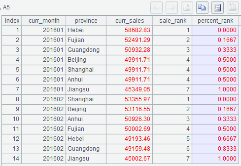
In order to achieve the same functionality of a window function, the above examples use lengthy, complicated SQL statements that are unreadable. To make matters worse, MySQL objects to the use of the implicit rule that multiple SELECT expressions should be calculated from left to right, which will lead to more complicated SQL statements. How to get a field value from the previous row without using the rule?
esProc, enabled by its distinctive Structured Process Language (SPL), can toss off the problem. It deals with the hardest job while leaving MySQL handling the basic SQL.
Let’s look at how esProc achieves the window function functionality with the SPL syntax.
1. SUM(), COUNT(), AVG(), MAX(), MIN() and VARIANCE
a)
select province, sales, sum(sales) over() `sum`,
    avg(sales) over() `avg`, max(sales) over() `max`,
    min(sales) over() `min`, count(*) over() `count`
from detail
where yearmonth=201601
order by sales;
| A | |
|---|---|
| 1 | =connect("mysql") |
| 2 | =A1.query@x("select * from detail where yearmonth=201601 order by sales desc") |
| 3 | =A2.sum(sales) |
| 4 | =A2.avg(sales) |
| 5 | =A2.max(sales) |
| 6 | =A2.min(sales) |
| 7 | =A2.count() |
| 8 | =A2.new(province, sales, A3:sum, A4:avg,A5:max,A6:min, A7:count) |
(1) Lines A3-A7 calculate sum, average, maximum value, minimum value and total number of rows over sales amounts;
(2) A8 creates a table sequence, where each row contains the total sale amount, average amount, max amount, min amount and total number of rows in the current month.
Below is A8’s result: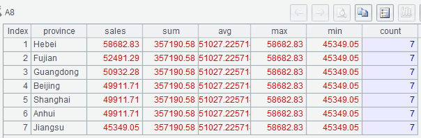
Now here’s the real challenge:
b)
select yearmonth,province,sales,
    sum(sales) over (partition by yearmonth) `sum`,
    avg(sales) over (partition by yearmonth) `avg`,
    max(sales) over (partition by yearmonth) `max`,
    min(sales) over (partition by yearmonth) `min`,
    count(*) over (partition by yearmonth) `count`
from detail
where yearmonth in (201601,201602) and sales>49500
order by yearmonth, sales desc;
| A | |
|---|---|
| 1 | =connect("mysql") |
| 2 | =A1.query@x("select * from detail where yearmonth in (201601,201602) and sales>49500 order by yearmonth,sales desc") |
| 3 | =A2.groups(yearmonth;sum(sales):sum,avg(sales):avg,max(sales):max,min(sales):min, count(1):count) |
| 4 | =A2.switch(yearmonth,A3) |
| 5 | =A4.new(yearmonth.yearmonth:yearmonth,province,sales,yearmonth.sum:sum, yearmonth.avg:avg,yearmonth.max:max,yearmonth.min:min,yearmonth.count:count) |
(1) A2 groups rows by month and calculates sum, average, maximum, minimum, and number of rows in the current month over sales amounts;
(2) A4 replaces each yearmonth field value in A2 with the record of corresponding month in A3.
Below is A5’s result: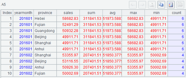
2.VARIANCE(), STD()
a)
select province, sales, variance(sales) over() `variance`, std(sales) over() `std`
from detail where yearmonth=201601;
| A | |
|---|---|
| 1 | =connect("mysql") |
| 2 | =A1.query("select * from detail where yearmonth=201601") |
| 3 | =A2.variance(sales) |
| 4 | =sqrt(A3) |
| 5 | =A2.new(province,sales,A3:variance,A4:std) |
(1)A3 calculates variance over sales amounts;
(2) A4 calculates A3’s square root to get the standard deviation.
Below is A5’s result: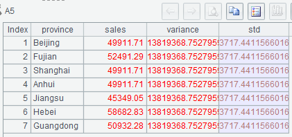
b)
select yearmonth, province, sales,
    variance(sales) over(partition by yearmonth) `variance`,
    std(sales) over(partition by yearmonth) `std`
from detail
where yearmonth in (201601, 201602);
| A | |
|---|---|
| 1 | =connect("mysql") |
| 2 | =A1.query@x("select * from detail where yearmonth in (201601,201602) order by yearmonth") |
| 3 | =A2.group(yearmonth) |
| 4 | =A3.new(yearmonth:m,~.variance(sales):v, sqrt(v):v2) |
| 5 | =A2.switch(yearmonth, A4:m) |
| 6 | =A5.new(yearmonth.m:yearmonth, province, sales, yearmonth.v:variance, yearmonth.v2:std) |
(1) A3 groups rows by month;
(2) A4 calculates the variance of sales amount in each month.
Below is A6’s result: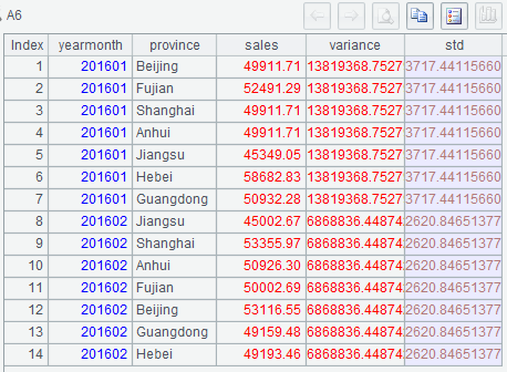
3.ROW_NUMBER(), RANK(), DENSE_RANK()and PERCENT_RANK()
a)
select province, sales, row_number() over(order by sales desc) `row_number`,
    rank() over (order by sales desc) `rank`,
    dense_rank() over (order by sales desc) `dense_rank`,
    percent_rank() over (order by sales desc) `percent_rank`
from detail
where yearmonth=201601;
| A | |
|---|---|
| 1 | =connect("mysql") |
| 2 | =A1.query("select * from detail where yearmonth=201601") |
| 3 | =A2.sort(sales:-1) |
| 4 | =A2.count() |
| 5 | =A3.new(province,sales,#:row_number,rank(sales):rank,ranki(sales):dense_rank, if(A4>1,(rank-1)/(A4-1),0):percent_rank) |
(1) In A5, the number sign # represents the sequence number of the current row in A3;
(2) The percentile rank is if(number of rows>1,(rank-1)/(number of rows-1),0).
Below is A5’s result: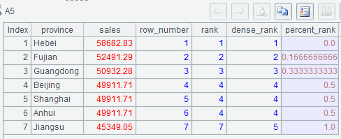
b)
select province, sales,
    row_number() over(partition by yearmonth order by sales desc)
        `row_number`,
    rank() over (partition by yearmonth order by sales desc) `rank`,
    dense_rank() over (partition by yearmonth order by sales desc)
        `dense_rank`,
    percent_rank() over (partition by yearmonth order by sales desc)
        `percent_rank`
from detail
where yearmonth in (201601,201602);
| A | |
|---|---|
| 1 | =connect("mysql") |
| 2 | =A1.query("select * from detail where yearmonth in (201601,201602)") |
| 3 | =A2.sort(yearmonth,sales:-1) |
| 4 | =A2.groups(yearmonth:m;count(1):count) |
| 5 | =A2.switch(yearmonth,A4:m) |
| 6 | =A3.new(yearmonth,province,sales,seq(yearmonth):row_number,rank(sales;yearmonth):rank, ranki(sales;yearmonth):dense_rank, if(yearmonth.count>1, (rank-1)/(yearmonth.count-1),0):percent_rank) |

4.NTILE()
a)
select province, sales, ntile(3) over() `ntile`
from detail
where yearmonth=201601;
| A | |
|---|---|
| 1 | =connect("mysql") |
| 2 | =A1.query("select * from detail where yearmonth in (201601,201602)") |
| 3 | =NumberOfBarrels=3 |
| 4 | =A2.count() |
| 5 | =A2.new(province,sales,z(#,NumberOfBarrels,A4):ntile) |
(1) A3 sets the number of barrels as 3;
(2) In A5, z(i,NumberOfBarrels,NumberOfRows) calculates the barrel number in the ith row.
Below is A5’s result: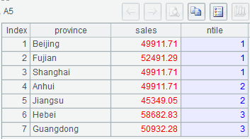
b)
select yearmonth, province, sales, ntile(3) over(partition by yearmonth) `ntile`
from detail
where yearmonth=201601 or( yearmonth=201602 and province!='Shanghai');
| A | |
|---|---|
| 1 | =connect("mysql") |
| 2 | =A1.query@x("select * from detail where yearmonth=201601 or (yearmonth=201602 and province!='Shanghai') order by yearmonth" ) |
| 3 | =NumberOfBarrels=3 |
| 4 | =A2.group(yearmonth:m;~.count():count) |
| 5 | =A2.switch(yearmonth,A4:m) |
| 6 | =A5.new(yearmonth.m:yearmonth,province,sales, z(seq(yearmonth),NumberOfBarrels,yearmonth.count):ntile) |
Below is A6’s result: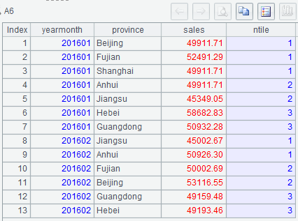
5.FIRST_VALUE(), LAST_VALUE(), NTH_VALUE(), LAG() and LEAD()
a)
select province,sales,
    first_value(sales) over(partition by yearmonth) `first_value`,
    last_value(sales) over(partition by yearmonth) `last_value`,
    nth_value(sales, 5) over(partition by yearmonth) `nth_value`,
    lag(sales, 2) over(partition by yearmonth) `lag`,
    lead(sales, 3) over(partition by yearmonth) `lead`
from detail
where yearmonth=201601;
| A | |
|---|---|
| 1 | =connect("mysql") |
| 2 | =A1.query@x("select * from detail where yearmonth=201601") |
| 3 | =A2.new(province, sales, A2.m(1).sales:first_value,A2.m(-1).sales:last_value, A2.m(5).sales:nth_value, ~[-2].sales:lag,~[3].sales:lead) |
(1) A2.m(i) gets the ith record in A2; it returns null if i exceeds the maximum number of rows, or (abs(i))th record if i is a negative value. Here A2(i) should not be used since error will be reported if i exceeds the maximum number.
Below is A3’s result: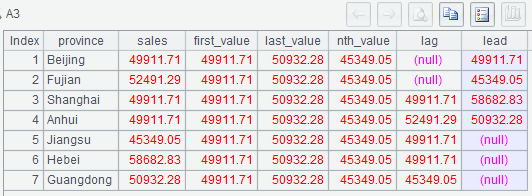
b)
select yearmonth,province,sales,
    first_value(sales) over(partition by yearmonth) `first_value`,
    last_value(sales) over(partition by yearmonth) `last_value`,
    nth_value(sales, 5) over(partition by yearmonth) `nth_value`,
    lag(sales, 2) over(partition by yearmonth) `lag`,
    lead(sales, 3) over(partition by yearmonth) `lead`
from detail
where yearmonth=201601 or (yearmonth=201602 and sales>50000);
| A | |
|---|---|
| 1 | =connect("mysql") |
| 2 | =A1.query@x("select * from detail where yearmonth=201601 or (yearmonth=201602 and sales>50000) order by yearmonth") |
| 3 | =A2.group(yearmonth:m;~.count():count,~.m(1).sales:first_value, ~.m(-1).sales:last_value,~.m(5).sales:nth_value) |
| 4 | =A2.switch(yearmonth, A3:m) |
| 5 | =A2.new(yearmonth.m:yearmonth, province, sales, yearmonth.first_value:first_value,yearmonth.last_value:last_value,yearmonth.nth_value:nth_value, (seq=seq(yearmonth),if(seq>2,~[-2].sales,null)):lag,if(yearmonth.count-seq>=3,~[3].sales,null):lead) |
(1) In A5, try not to use expression seq(yearmonth) within the if function. As seq() function loops through records in A2 to calculate a cumulative value, it will miss a value if it skips a loop;
(2) In A5, expression seq=seq(yearmonth) assigns a value to variable seq; thus an expression after it can directly reference the variable.
Below is A5’s result: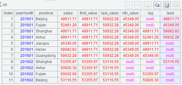
6. CUME_DIST()
a)
select province,sales, cume_dist() over(order by sales) `cume_dist`
from detail
where yearmonth=201601;
| A | |
|---|---|
| 1 | =connect("mysql") |
| 2 | =A1.query@x("select * from detail where yearmonth=201601 order by sales desc") |
| 3 | =A2.count() |
| 4 | =A2.new(province,sales,(A3-rank(sales)+1)/A3:cume_dist) |
| 5 | =A4.rvs() |
(1) Expression CUME_DIST() over (order by sales) calculates the cumulative distribution of sales amounts in ascending order. The formula is this: number of rows where the sales is less than or equal to the current sales/total number of rows;
(2) Number of rows where sales is less than or equal to the current sales = total number of rows – rank of the current sales ranked in descending order + 1;
(3) In A2, sales amounts should be ordered in descending order;
(4) A5 sorts data in a reverse order.
Below is A5’s result: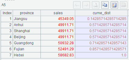
b)
select yearmonth, province,sales,
    cume_dist() over(partition by yearmonth order by sales) `cume_dist`
from detail
where yearmonth in (201601,201602);
| A | |
|---|---|
| 1 | =connect("mysql") |
| 2 | =A1.query@x("select * from detail where yearmonth in (201601,201602) order by yearmonth desc,sales desc") |
| 3 | =A2.groups(yearmonth:m;count(1):count) |
| 4 | =A2.switch(yearmonth,A3:m) |
| 5 | =A2.new(yearmonth.m:yearmonth,province,sales,(yearmonth.count-rank(sales;yearmonth)+1)/yearmonth.count:cume_dist) |
| 6 | =A5.rvs() |
(1) As data will be re-sorted in a reverse order, A2 orders sales amounts by month in descending order.
Below is A6’s result: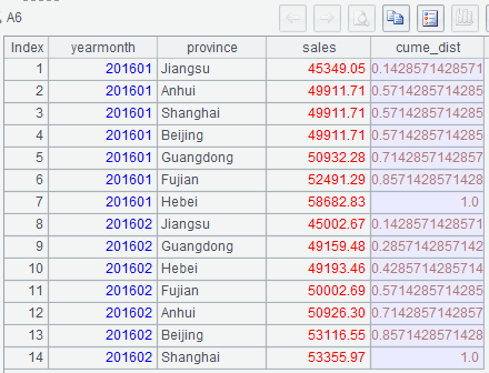
In these examples, with grid-style code, esProc handles calculations step by step in a natural, intuitive and effortless way. You can look up the query result for each step and finish the whole script more easily.
SPL Official Website 👉 http://www.scudata.com
SPL Feedback and Help 👉 https://www.reddit.com/r/esProc
SPL Learning Material 👉 http://c.scudata.com
SPL Source Code and Package 👉 https://github.com/SPLWare/esProc
Discord 👉 https://discord.gg/ydhVnFH9
Youtube 👉 https://www.youtube.com/@esProc_SPL