What should I do when it is difficult to write complex SQL in Java reporting tools?
To other questions:
What should I do when the data source in the Java report tool cannot be calculated by SQL?
How to handle multi-source calculations in Java reporting tools?
Solution: esProc – the professional computational package for Java

esProc is a class library dedicated to Java-based calculations and aims to simplify Java code. SPL is a scripting language based on the esProc computing package. It can be deployed together with Java programs and understood as a stored procedure outside the database. Its usage is the same as calling a stored procedure in a Java program. It is passed to the Java program for execution through the JDBC interface, realizing step-by-step structured computing, return the ResultSet object.
Some databases, such as MySQL, don’t have powerful analytic functions. Some others, such as Vertica, don’t support stored procedures. Instead, we turn to external languages to deal with complicated data computations. If we directly use Java to implement similar SQL functions and the stored procedure function, write lengthy code for a certain computing requirement. The code is almost impossible to reuse.
It’s not easy to implement complicated logic, even with analytic functions. So here’s a common computing task: Find the first N customers whose sales account for half of the total sum and sort them by the amount in descending order. Oracle implements it this way:
with A as
(selectCUSTOM,SALESAMOUNT,row_number() over (order by SALESAMOUNT) RANKING
from SALES)
select CUSTOM,SALESAMOUNT
from (select CUSTOM,SALESAMOUNT,sum(SALESAMOUNT) over (order by RANKING) AccumulativeAmount
from A)
where AccumulativeAmount>(select sum(SALESAMOUNT)/2 from SALES)
order by SALESAMOUNT desc
The Oracle script sorts records by sales amount in ascending order and then finds the customers whose sales amount to half of the total sum in the opposite direction according to the condition that the accumulated amount is greater than half of the entire sum. To avoid the window function’s mistake in handling the same sales amounts when calculating the accumulated value, we calculate the sales amounts rankings in the first subquery.
Here is the code to implement the same logic using SPL:
| A | B | |
|---|---|---|
| 1 | =connect("verticaLink") | /Connect to Vertica database |
| 2 | =A1.query("select * from sales").sort(SALESAMOUNT:-1) | /Get the sales records and sort them by sales amount in descending order |
| 3 | =A2.cumulate(SALESAMOUNT) | /Calculate a sequence of accumulated values; the function is a replacement of database window function |
| 4 | =A3.m(-1)/2 | /Calculate half of total sales amount |
| 5 | =A3.pselect(~>=A4) | /Find the position in the accumulated value sequence where half of total sales amount falls |
| 6 | =A2(to(A5)) | /Get the record where half of total sales amount falls and records before it |
| 7 | >A1.close() | /Close database connection |
| 8 | return A6 | /Return A6’s result |
From the above code, we can see that SPL uses a set of concise syntax to replace the logic that needs to be nested SQL+window functions and has universal consistency (any data source code is consistent)
The integration of SPL and Java report development tools is also very simple. Take Vertica as the data source and Birt as the reporting tool as an example. Copy the esProc core jar package and the corresponding database driver jar package to the Birt development environment [installation directory]\plugins\org.eclipse.birt.report.data.oda.jdbc_4.6.0.v20160607212 (different Birt versions are slightly different) .
Create a new report in the Birt development tool and add the esProc data source “esProcConnection”

Birt calls the Vertica external stored procedure (esProc data set). Create a new “Data Sets”, select the configured esProc data source (esProcConnection), and select the data set type to select a stored procedure (SQL Stored Procedure Query).

Query Text input: {call VerticaExternalProcedures()}, where VerticaExternalProcedures is the SPL script file name

Finish, preview the data (Preview Results)

For more Java report integration details, please refer to: How to Call an SPL Script in BIRT and How to Call an SPL Script in JasperReport
SQL is not good at mainly including complex set calculations, ordered calculations, associative calculations, and multi-step calculations. SQL collection is not thorough enough, and there is no explicit collection data type, which makes it difficult to reuse the collection generated during the calculation process. For example, after grouping, it must be mandatory to summarize. It cannot calculate the subset based on the group itself and does not support multi-step code, and often forces programmers to write long statements with several levels of nesting. Although stored procedures can solve this problem to a certain extent, sometimes the actual environment does not allow us to use stored procedures. For example, DBA strictly controls the database procedure permissions. Old databases and small databases do not support stored procedures, etc., and the debugging of stored procedures is also very inconvenient. Therefore, it is not very suitable for writing calculations with stored procedures.
SPL is a professional structured computing language. It is designed based on ordered sets and provides complete set operations. It is equivalent to the combination of the advantages of Java and SQL. It is good at simplifying SQL complex operations. Problems like ordered calculations are very easy. Let me give you a few more examples of different types.
Simplify SQL Grouping
According to Employee table (Below is a part of it), calculate the average salary for each state of [California, Texas, New York, Florida] and for all the other states as a whole, which are classified as “Other”.
ID |
NAME |
BIRTHDAY |
STATE |
DEPT |
SALARY |
1 |
Rebecca |
1974/11/20 |
California |
R&D |
7000 |
2 |
Ashley |
1980/07/19 |
New York |
Finance |
11000 |
3 |
Rachel |
1970/12/17 |
New Mexico |
Sales |
9000 |
4 |
Emily |
1985/03/07 |
Texas |
HR |
7000 |
5 |
Ashley |
1975/05/13 |
Texas |
R&D |
16000 |
… |
… |
… |
… |
… |
… |
SQL:
with cte1(ID,STATE) as
      (select 1,'California' from DUAL
         UNION ALL select 2,'Texas' from DUAL
         UNION ALL select 3,'New York' from DUAL
         UNION ALL select 4,'Florida' from DUAL
         UNION ALL select 5,'OTHER' from DUAL)
   select
      t1.STATE, t2.AVG_SALARY
   from cte1 t1
   left join
      (select
         STATE,avg(SALARY) AVG_SALARY
      from
         ( select
            CASE WHEN
            STATE IN ('California','Texas','New York','Florida')
            THEN STATE
            ELSE 'OTHER' END STATE,
            SALARY
         from EMPLOYEE)
      group by STATE) t2
   on t1.STATE=t2.STATE
   order by t1.ID
SPL:
SPL has A.align() function to do this. It uses @n option to put the non-matching members into a new group.
A |
|
1 |
=T("Employee.csv") |
2 |
[California,Texas,New York,Florida] |
3 |
=A1.align@an(A2,STATE) |
4 |
=A3.new(if (#>A2.len(),"OTHER",STATE):STATE,~.avg(SALARY):AVG_SALARY) |
A1: Import Employee table.
A2: Define a constant set of regions.
A3: A.align() groups Employee table according to A2’s set of states. @a option is used to return all matching members for each group; @n option enables putting the non-matching members into a new group.
A4: Name the new group “OTHER” and calculate the average salary of each group.
SQL uses JOIN to achieve an alignment grouping because it does not have a method to do it directly. As a SQL result set is unordered, we record the order of the records in the original table through their original row numbers. This makes SQL solution to an alignment grouping problem complicated. SPL offers A.align() function for specifically handling alignment grouping operations, which features concise syntax and efficient execution.
Simplify SQL Join
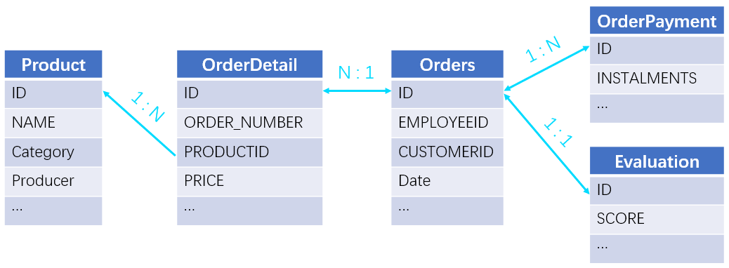
Get order information of the year 2014 (order IDs, product names and total amounts) where the product name contains “water” and order amount is greater than 200, and that do not pay in installment and get 5-star evaluation. Below is part of the source data and the relationships between tables:
SQL:
This task involves one-to-many relationship, many-to-one relationship and one-to-one relationship. It is wrong to join them all with the JOIN operation because that will result in many-to-many relationship. The right way is to handle the many-to-one relationship (foreign key table) first by attaching foreign key values or desired field values to the table at the “many” end, and we have one-to-one relationship and one-to-many relationship only. Then we group the sub table by the primary table’s primary key (order ID), which makes the key the sub table’s actual primary key. Finally, we join the four tables through order ID. Below are SQL statements:
SELECT
      Orders.ID,Detail1.NAME, Detail1.AMOUNT
   FROM (
      SELECT ID
      FROM ORDERS
      WHERE
         EXTRACT (YEAR FROM Orders.ORDER_DATE)=2014
   ) Orders
   INNER JOIN (
      SELECT ID,NAME, SUM(AMOUNT) AMOUNT
      FROM (
         SELECT
            Detail.ID,Product.NAME,Detail.PRICE*Detail.COUNT AMOUNT
         FROM ORDER_DETAIL Detail
         INNER JOIN
         PRODUCT Product
         ON Detail.PRODUCTID=Product.ID
         WHERE NAME LIKE '%water%'
      )
      GROUP BY ID,NAME
   ) Detail1
   ON Orders.ID=Detail1.ID
   INNER JOIN(
      SELECT
         DISTINCT ID
      FROM ORDER_PAYMENT
      WHERE INSTALMENTS=0
   ) Payment
   ON Orders.ID = Payment.ID
   INNER JOIN(
      SELECT ID
      FROM EVALUATION
      WHERE SCORE=5
   ) Evaluation
   ON Orders.ID = Evaluation.ID
The SQL statements are difficult to write, hard to understand and maintain. More importantly, it is inconvenient to check whether the statements are correctly written since there are too many joins and nested queries.
SPL:
A |
|
1 |
=T("Orders.txt").select(year(ORDER_DATE)==2014) |
2 |
=T("Product.txt").select(like(NAME, "*water*")) |
3 |
=T("OrderDetail.txt").switch@i(PRODUCTID, A2:ID) |
4 |
=A3.group(ID).select(sum(PRICE*COUNT)>200) |
5 |
=T("OrderPayment.txt").select(INSTALMENTS==0).group(ID) |
6 |
=T("Evaluation.txt").select(SCORE==5) |
7 |
=join(A1:Orders,ID;A4:Detail,ID;A5:Payment,ID;A6:Evaluation,ID) |
8 |
=A7.new(Orders.ID,Detail.PRODUCTID.NAME,Detail.sum(PRICE*COUNT):AMOUNT) |
A1: Import Orders table and select records of the year 2014.
A2: Import Product table and select records that contain water.
A3: Import OrderDetail table and objectify the foreign key PRODUCTID by replacing its values with corresponding records in Product table.
A4: Group OrderDetail table by ID field and select records where the amount is above 200.
A5: Import OrderPayment table and select records that do not have installment information.
A6: Import Evaluation table and select records containing 5-star evaluations.
A7: The join() function joins Orders table, OrderDetail table, OrderPayment table, and Evaluation table according to ID fields.
A8: Return the eligible order IDs, product names and order amounts.
The SPL script has two more lines of code. The import, select, and group operations on each table are separately performed, and only one line (A7) is for the join. The logic is natural and clear.
Simplify SQL Transposition
Based on the following channel-based sales table, generate a new table storing information by date. Below is part of the source table:
YEAR |
MONTH |
ONLINE |
STORE |
2020 |
1 |
2440 |
3746.2 |
2020 |
2 |
1863.4 |
448.0 |
2020 |
3 |
1813.0 |
624.8 |
2020 |
4 |
670.8 |
2464.8 |
2020 |
5 |
3730.0 |
724.5 |
… |
… |
… |
… |
Below is the result of expected layout:
CATEGORY |
1 |
2 |
3 |
… |
ONLINE |
2440 |
1863.4 |
1813.0 |
… |
STORE |
3746.2 |
448.0 |
624.8 |
… |
We need to perform both row-to-column transposition and column-to-row transposition to get this done. First, we perform column-to-row transposition to transform channel types into values under CATEGORY field:
YEAR |
MONTH |
CATEGORY |
AMOUNT |
2020 |
1 |
ONLINE |
2440 |
2020 |
1 |
STORE |
3746.2 |
2020 |
2 |
ONLINE |
1863.4 |
2020 |
2 |
STORE |
448.0 |
… |
… |
… |
… |
Then we perform row-to-column transposition to convert MONTH values into column names. The complete SQL query is as follows:
SELECT *
   FROM (
      SELECT *
      FROM MONTH_SALES
      UNPIVOT (
         AMOUNT FOR CATEGORY IN (
            "ONLINE",STORE
         )
      )
      WHERE YEAR=2020
   )
   PIVOT (
      MAX(AMOUNT) FOR MONTH
      IN (
         1 AS "1",2 AS "2",2 AS "3",
         4 AS "4",5 AS "5",6 AS "6",
         7 AS "7",8 AS "8",9 AS "9",
         10 AS "10",11 AS "11",12 AS "12"
      )
   )
SQL does not support using a non-constant expression as PIVOT/UNPIVOT value, so all months need to be enumerated for the row-to-column transposition.
SPL:
According to the natural logic, SPL handles the task using A.pivot@r() and A.pivot() respectively for column-to-row transposition and row-to-column transposition:
A |
|
1 |
=T("MonthSales.csv").select(YEAR:2020) |
2 |
=A1.pivot@r(YEAR,MONTH; CATEGORY, AMOUNT) |
3 |
=A2.pivot(CATEGORY; MONTH, AMOUNT) |
A1: Import MonthSales table and select records of the year 2020.
A2: A1.pivot@r() performs column-to-row transposition to convert channel types into values of CATEGORY field.
A3: A2.pivot () performs row-to-column transposition to transform MONTH field values into column names.
Both SQL and SPL handle simple transposition scenarios well. The issue is that the real-world situations cannot always dealt with using the mode of grouping & aggregation plus PIVOT. In the subsequent essays in our transposition series, we will introduce how the two languages handle complicated static transpositions and dynamic transpositions.
Simplify SQL Recursion
According to a company’s organizational structure below, get Beijing Branch Office’s subordinate organizations and its superiors’ names (separate multilevel organizations by comma).
ID |
ORG_NAME |
PARENT_ID |
1 |
Head Office |
0 |
2 |
Beijing Branch Office |
1 |
3 |
Shanghai Branch Office |
1 |
4 |
Chengdu Branch Office |
1 |
5 |
Beijing R&D Center |
2 |
… |
… |
… |
SQL:
The first idea for doing this is that, during the recursive process for searching for the superiors for each organization, stop the recursion if the specified value (the Beijing Branch Office) is found, keep its records and filter away records of the organizations that cannot be found. It is difficult for SQL to hit the target with one round of recursion. So we divide the task into two steps. First, find all subordinate organizations of Beijing Branch Office; second, as the solution to the above problem does, find all superior organizations for each of those organizations until Beijing Branch Office appears. Below is the SQL queries:
WITH CTE1 (ID,ORG_NAME,PARENT_ID) AS(
   SELECT
      ID,ORG_NAME,PARENT_ID
   FROM ORGANIZATION
   WHERE ORG_NAME='Beijing Branch Office'
   UNION ALL
   SELECT
      ORG.ID,ORG.ORG_NAME,ORG.PARENT_ID
   FROM ORGANIZATION ORG
   INNER JOIN CTE1
   ON ORG.PARENT_ID=CTE1.ID
)
,CTE2 (ID,ORG_NAME,PARENT_ID,O_ID,GROUP_NUM) AS(
   SELECT
      ID,ORG_NAME,PARENT_ID,ID O_ID,1 GROUP_NUM
   FROM CTE1
   UNION ALL
   SELECT ORG.ID,ORG.ORG_NAME,ORG.PARENT_ID,
      CTE2.O_ID,CTE2.GROUP_NUM+1 GROUP_NUM
   FROM ORGANIZATION ORG
   INNER JOIN CTE2
   ON ORG.ID=CTE2.PARENT_ID AND
   CTE2.ORG_NAME<>'Beijing Branch Office'
)
SELECT
   MAX(O_ID) ID, MAX(O_ORG_NAME) ORG_NAME,
   MAX(PARENT_NAME) PARENT_NAME
FROM(
   SELECT
      O_ID, O_ORG_NAME,
      WM_CONCAT(ORG_NAME) OVER
      (PARTITION BY O_ID ORDER BY O_ID,GROUP_NUM) PARENT_NAME
   FROM(
      SELECT
         ID,PARENT_ID,O_ID,GROUP_NUM,
         CASE WHEN GROUP_NUM=1 THEN NULL ELSE ORG_NAME END ORG_NAME,
         CASE WHEN GROUP_NUM=1 THEN ORG_NAME ELSE NULL END O_ORG_NAME
      FROM (
         SELECT
            ID,ORG_NAME,PARENT_ID,O_ID,GROUP_NUM,ROWNUM RN
         FROM CTE2
         ORDER BY O_ID,GROUP_NUM
      )
   )
)
GROUP BY O_ID
ORDER BY O_ID
With Oracle, you can also use START WITH … CONNECT BY … PRIOR … to do the recursive query, as shown below:
WITH CTE1 AS (
   SELECT ID,ORG_NAME,PARENT_ID,ROWNUM RN
   FROM ORGANIZATION ORG
   START WITH ORG.ORG_NAME='Beijing Branch Office'
   CONNECT BY ORG.PARENT_ID=PRIOR ORG.ID
)
,CTE2 AS (
   SELECT
      ID,ORG_NAME,PARENT_ID,RN,
      CASE WHEN LAG(ORG_NAME,1) OVER(ORDER BY RN ASC)= 'Beijing Branch Office' OR
      LAG(ORG_NAME,1) OVER(ORDER BY RN ASC) IS NULL THEN 1 ELSE 0 END FLAG
   FROM(
      SELECT ID,ORG_NAME,PARENT_ID,ROWNUM RN
      FROM CTE1
      START WITH 1=1
      CONNECT BY CTE1.ID=PRIOR CTE1.PARENT_ID
   )
)
SELECT
   MAX(ID) ID, MAX(O_ORG_NAME) ORG_NAME,
   MAX(PARENT_NAME) PARENT_NAME
FROM(
   SELECT
      ID,O_ORG_NAME,GROUP_ID,
      WM_CONCAT(ORG_NAME) OVER
      (PARTITION BY GROUP_ID ORDER BY RN) PARENT_NAME
   FROM(
      SELECT
         ID, ORG_NAME, O_ORG_NAME,RN,
         SUM(ID) OVER (ORDER BY RN) GROUP_ID
      FROM(
         SELECT
            PARENT_ID,RN,
            CASE WHEN FLAG=1 THEN NULL ELSE ORG_NAME END ORG_NAME,
            CASE WHEN FLAG=1 THEN ID ELSE NULL END ID,
            CASE WHEN FLAG=1 THEN ORG_NAME ELSE NULL END O_ORG_NAME
         FROM CTE2
      )
   )
)
GROUP BY GROUP_ID
ORDER BY GROUP_ID
SPL:
SPL offers A.prior(F,r) function to do the recursive query to find the refences until a specific value appears:
A |
|
1 |
=T("Organization.txt") |
2 |
>A1.switch(PARENT_ID,A1:ID) |
3 |
=A1.select@1(ORG_NAME=="Beijing Branch Office") |
4 |
=A1.new(ID,ORG_NAME,~.prior(PARENT_ID,A3) :PARENT_NAME) |
5 |
=A4.select(PARENT_NAME!=null) |
6 |
=A5.run(PARENT_NAME=PARENT_NAME.(PARENT_ID.ORG_NAME).concat@c()) |
A1: Import the Organization table.
A2: Objectify the ID foreign key of the superior organization to convert it into the corresponding record and achieve foreign key objectification.
A3: Get records of Beijing Branch Office.
A4: Create a new table made up of ID, organization name and the set of records of all superior organizations.
A5: Get records that has at least one superior organization, that is, those of Beijing Branch Office.
A6: Join up names of superior organizations into a comma-separated string in a circular way.
The SPL solution is logically clear and concise. It uses records of Beijing Branch Office as parameters to do the recursive search of references.
More SQL Comparisons
Refer to Use SPL in applications - Comparison with SQL
SPL Official Website 👉 http://www.scudata.com
SPL Feedback and Help 👉 https://www.reddit.com/r/esProc
SPL Learning Material 👉 http://c.scudata.com
SPL Source Code and Package 👉 https://github.com/SPLWare/esProc
Discord 👉 https://discord.gg/ydhVnFH9
Youtube 👉 https://www.youtube.com/@esProc_SPL