

Multipurpose traversal of SPL
Principle of multipurpose traversal
When traversing the data table on external storage, most of the time is spent on reading data from the hard disk. Therefore, we would hope to do as many things as possible over a single reading, that is, the data read out during the traversal process can be used to the maximum extent.
For example, we hope to perform two calculations when grouping and aggregating the orders table. The first one (compute1) is to count the sales by product group to get the result (result1), and the second one (compute2) is to count the maximum order amount of each area to get the result (result2). To get the two results, a direct way is to traverse twice, which is roughly as shown in Figure 1 below:
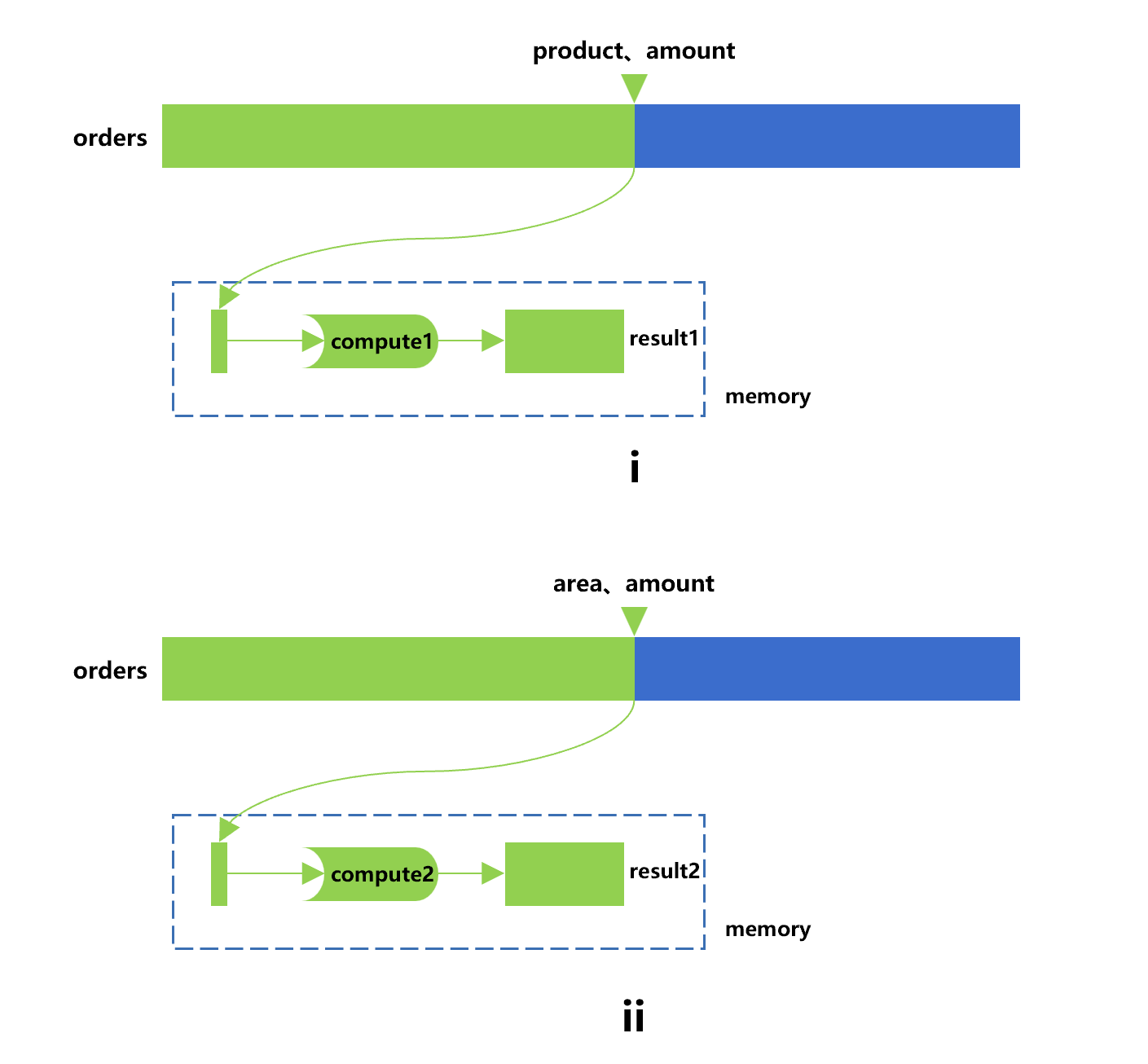
Figure 1: Traverse twice
Step i in this drawing is to use the cursor to traverse the orders table to fetch out the product and amount fields, and get result1 following the compute1; Step ii is to use a new cursor to traverse once again the orders table to fetch out the area and amount fields, and then get the result2 after the compute2 is performed.
If the orders table adopts the columnar storage, the amount field will be repeatedly read in two traversals. In case the data in the orders are stored in row-based storage mode, the amount of data read repeatedly will be larger.
To reduce the amount of data read, we use some skills, which allow us to get two grouped results by only traversing the orders once. The SPL code is roughly as follows:
A |
|
1 |
=file("orders.ctx").open() |
2 |
=A1.cursor(area,product,amount).groups(area,product;sum(amount):samount,max(amount):mamount) |
3 |
=A2.groups(product;sum(samount)) |
4 |
=A2.groups(area;max(mamount)) |
In this way, although more amount of computation will be performed by CPU and more memory space will be occupied since there is a need to calculate and keep a more detailed grouped result set, the traversal amount will be much less, and hence a better performance can usually be obtained.
However, if we want to do different grouping and aggregating on more fields, the code will be much more cumbersome; If we want to do some operations, exclusive of simple grouping, on this cursor, such as filtering followed by grouping, it is almost impossible to code with such techniques. Using SQL in the database will face this dilemma.
SPL provides a more powerful multipurpose traversal technology to solve such problems. For ease of understanding, let's first look at the process of performing compute1by using only the cursor, basically as shown in Figure 2 below:
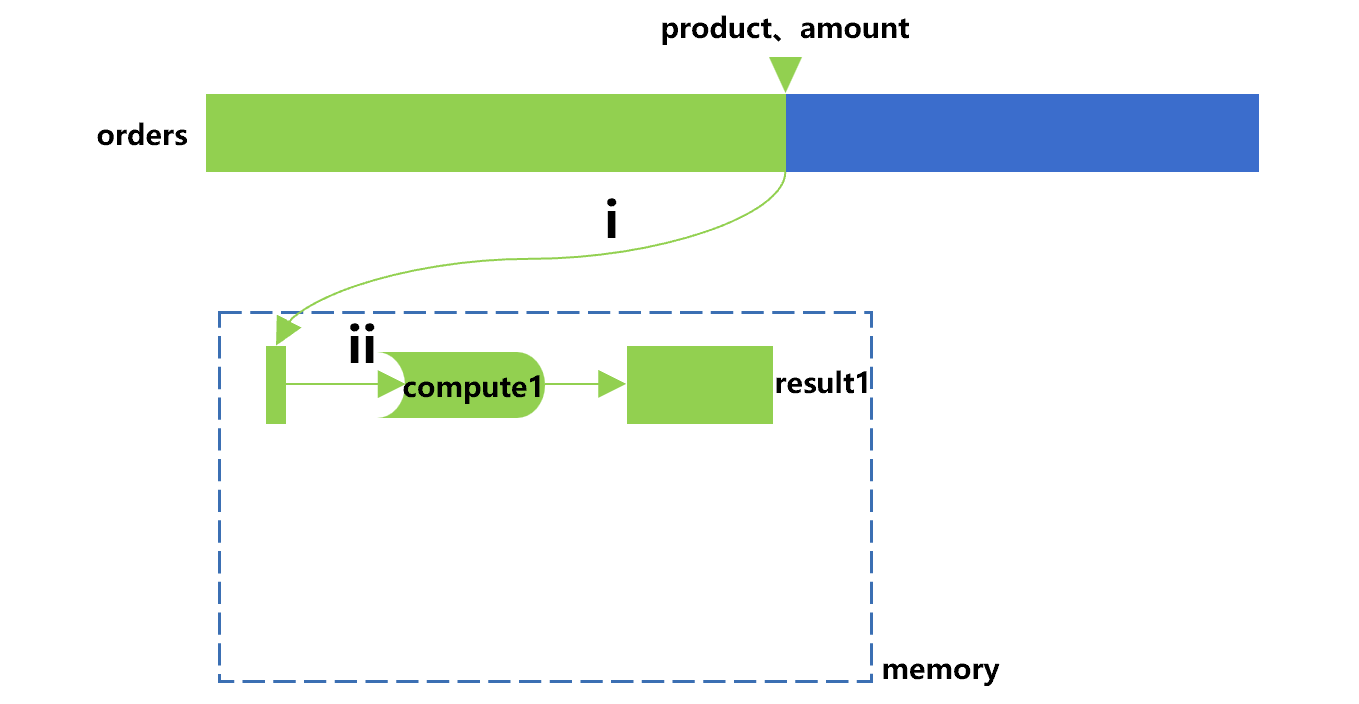
Figure 2 Performing compute1 by using only the cursor
In this drawing, the cursor will actively do action i to perform the calculation defined on it, that is, fetching out the product and amount fields from the orders table in batches. Action ii is to sum the amount by the product group, that is, performing compute1 for this batch of order data. The cursor will keep repeating the two actions until the traversal ends and the result1 is obtained.
The corresponding SPL code is as follows:
A |
|
1 |
=file("orders.ctx").open() |
2 |
=A1.cursor(area,product,amount) |
3 |
=A2.groups(product;sum(amount)) |
A3 defines compute1.
Next, we can regard compute1 performed by the cursor as a main line and reuse the traversal on this basis. The general process is shown in Figure 3:

Figure 3: Multipurpose traversal
In Figure 3, in addition to the main line of compute1 performed on the cursor, we add a bypass to perform compute2. In the process of performing the calculation (i.e., compute1), the cursor will fetch out a batch of order data from the orders table each time. If the cursor finds that there exists a bypass, it will send this batch of data to the bypass, that is, action iii, and then perform the compute2, the calculation result will be temporarily stored.
We call this bypass (compute2 and stored result) a channel synchronized with the cursor. In this way, the cursor also traverses the orders after compute1 is performed. The cursor operation itself will return result1, and we can also obtain result2 in the bypass channel, which can be taken out through action iv when needed.
By comparing figure 3 and figure 1, we find that the amount of computation on CPU in multipurpose traversal is the same as that in traversing twice, both cases only need to do two small grouping. However, the reading amount of hard disk of the former is much less than the latter, and the amount field is read only once.
The SPL code corresponding to multipurpose traversal is as follows:
A |
|
1 |
=file("orders.ctx").open() |
2 |
=A1.cursor(product,area,amount) |
3 |
=channel(A2).groups(area;max(amount)) |
4 |
=A2.groups(product;sum(amount)) |
5 |
=A3.result() |
Compared with the code with only cursor, this code adds A3 and A5.
A3 uses the channel function to define a channel synchronized with cursor A2, on which compute2 is attached.
A5 is to take out the result temporarily stored in the channel to get result2, corresponding to step iv in Figure 3.
The multipurpose traversal mechanism works for all cursors, not just the composite table.
A cursor can define multiple synchronous channels and attach multiple sets of calculations at the same time. Moreover, such calculations can be written at will, not just the grouping, and can also be written in multiple steps. For example, we can add one more calculation (compute3) to first filter out orders with an amount of over 50, and then count the number of records. Refer to Figure 4 below for the calculation process:
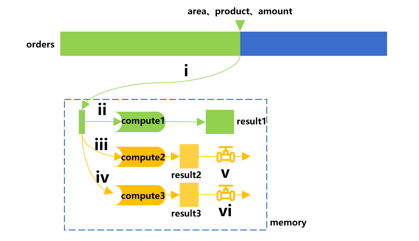
Figure 4 Adding a calculation (compute3)
In this figure, on the basis of the original one cursor and one channel, another bypass is added to calculate computer3.
The corresponding SPL code is roughly as follows after adding computer3:
A |
B |
|
1 |
=file("orders.ctx").open() |
|
2 |
=A1.cursor(product,area,amount) |
|
3 |
=channel(A2).groups(area;max(amount)) |
|
4 |
=channel(A2).select(amount>=50).total(count(1)) |
|
5 |
=A2.groups(product;sum(amount)) |
|
6 |
=A3.result() |
=A4.result() |
A4 uses the channel function to define the second channel synchronized with cursor A2, on which computer3 is attached.
When traversing the cursor in A5 to calculate compute1, the read data will be sent to channel A4 at the same time to do compute3. After the traversal, the corresponding calculation result will be kept in channel A4, which can be taken out in B5.
In fact, the calculation (computer1) of the cursor itself can also be done with the channel, and the cursor itself only does the traversal. In this way, the status of multiple calculations is equal, and the code will appear more symmetrical:
A |
B |
|
1 |
=file("orders.ctx").open() |
|
2 |
=A1.cursor(product,area,amount) |
|
3 |
=channel(A2).groups(product;sum(amount)) |
|
4 |
=channel(A2).groups(area;max(amount)) |
|
5 |
=channel(A2).select(amount>=50).total(count(1)) |
|
6 |
=A2.skip() |
=A3.result() |
7 |
=A4.result() |
=A5.result() |
From A3 to A5, use the channel function to define three channels synchronized with cursor A2, and attach three calculations (compute1 to compute3) respectively.
When the cursor is traversed in A6, the read data will also be sent to the three channels at the same time. After the traversal is over, the corresponding calculation results will be kept in three channels, which can be taken out in B6, A7, and B7.
This situation is quite common. SPL provides a special statement-pattern channel syntax. The above code can also be written as follows:
A |
B |
|
1 |
=file("orders.ctx").open() |
|
2 |
=A1.cursor(product,area,amount) |
|
3 |
cursor A2 |
=A3.groups(product;sum(amount)) |
4 |
cursor |
=A4.groups(area;max(amount)) |
5 |
cursor |
=A5.select(amount>=50).total(count(1)) |
6 |
||
After the cursor is created in A2, use the cursor statement in A3 to create a channel for it, and attach an operation on it. We can create multiple channels, if the cursor parameters are not written in the subsequent statements, it indicates the same cursor will be used.
After all cursor statements (code blocks) are written, SPL will consider that all channels have been defined completely, and will start traversing the cursor, calculate the operation results of each channel and store them in the cell where the cursor statement is located.
Here, B3, B4 and B5 respectively define compute1, compute2 and compute3. These calculation results will be placed in A3, A4, and A5 respectively (note that it is not B3, B4, B5).
Multipurpose traversal for data split
The idea of multi-purpose traversal can be applied to data split. For example, there is a large text file “data.txt” from which we hope to pick out the correct data (meeting the given conditions) to do further analysis, in this case, using the select function of the cursor works. Meanwhile, we may also want to know what the error data (failing to meet the conditions) are, so as to prevent this from happening again. Since one-time filtering cannot separate the records that meet and do not meet the conditions at the same time, in this case, the multi-purpose traversal technology can be used. The rough calculation process is shown in Figure 5:
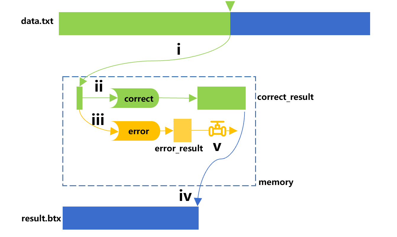
Figure 5 Data split
In Figure 5, the cursor defines the select function to do conditional filtering, that is, calculating the "correct” to get the correct data correct_result, and output it to result.btx. The channel of the cursor defines an opposite condition, that is, calculating the "error" to get the error data error_ result. Here we assume that there are few records that do not satisfy the condition and can be stored in memory.
The corresponding SPL code is as follows:
A |
|
1 |
=file("data.txt").cursor@t() |
2 |
… |
3 |
=channel(A1).select(!(${A2})).fetch() |
4 |
=A1.select(${A2}) |
5 |
>file("result.btx").export@b(A4) |
6 |
=A3.result() |
When the filter condition is filled in A2, the channel in A3 will calculate the “error” to filter out records that do not meet the conditions, and fetch the error_result.
The cursor in A4 performs the calculation "correct", filtering out the correct records that meet the condition.
A5 traverses the cursor and writes the records that meet the conditions into a new file, corresponding to step iv in Figure 5.
A6 can take out the channel result, corresponding to step v in Figure 5.
However, doing so still needs to calculate this condition twice (records that meet and do not meet the condition to be calculated separately). SPL provides a method directly in its select function, which can take out the records that do not meet the condition at the same time, but such records can only be written to another file, and only in the format of bin file.
A |
|
1 |
=file("data.txt").cursor@t() |
2 |
… |
3 |
=A1.select(${A2};file("error.btx")) |
4 |
>file("result.btx").export@b(A3) |
Similarly, we may also split the big data table into multiple groups. For example, split the order records into multiple files by region for distribution purpose, in this case, the channel can also be used. However, the number of channels needs be predetermined in the code, and we should know how many channels are needed in advance since we cannot temporarily create a new channel in the process of grouping.
To solve this problem, SPL attaches a function that can split and write-to-files in performing the sequence number group on the cursor. For example, the following code divides the orders into 12 months (taking the month as example is because it is easy to do sequence-numberization; for other cases, you can do sequence-numberization yourself).
A |
|
1 |
=file("orders.txt").cursor@t() |
2 |
=12.(file("order"/~/".btx")) |
3 |
=A1.groupn(month(dt);A2) |
4 |
=A1.skip() |
The groupn() function in this code is a delayed cursor, which merely records the action, and will be actually calculated during cursor traversal. We should prepare a corresponding number of file objects (A2) in advance. Similar to select(), groupn() can only write data as bin files.
SPL Official Website 👉 http://www.scudata.com
SPL Feedback and Help 👉 https://www.reddit.com/r/esProc
SPL Learning Material 👉 http://c.scudata.com
SPL Source Code and Package 👉 https://github.com/SPLWare/esProc
Discord 👉 https://discord.gg/ydhVnFH9
Youtube 👉 https://www.youtube.com/@esProc_SPL


Chinese version