Wide table abounds in BI business. Whenever building a BI system, the first thing you need to do is to prepare a wide table. Sometimes the wide table in the system may have hundreds of fields, splitting this table is often needed due to “too wide” exceeding the limit on the number of fields of database table.

Why are people so keen on creating wide table? There are two main reasons.

One is to improve query performance. Usually, modern BI takes relational database as backend, yet the computing performance of HASH JOIN algorithm that SQL usually adopts will decrease sharply when the number of tables and levels to be associated increases, and this phenomenon can be observed when there are only seven or eight tables and three or four levels. However, the association complexity in BI business far exceeds this scale, it will fail to meet the query requirement for obtaining the result instantly at the front end if a query task is performed directly with SQL’s JOIN algorithm. In order to avoid performance problem caused by association, it needs to eliminate association from query stage, that is, associate multiple tables in advance and store them in a single table (i.e., wide table). In this way, there is no need to associate again when querying, the query performance is thus improved.

The other is to reduce business difficulty. Sinceit is very difficult to express and use multi-table association, especially the complex association, at BI front-end, if automatic association is adopted (match based on information like field type), the system will get confused when facing fields of the same dimension (e.g., a table has more than 2 area fields), and does not know which field should be associated. Similarly, it is also hard to handle the cycle association between tables or self-association at frond-end; If many tables are presented open to users, allowing them to associate by themselves, it is almost useless because they cannot understand the relationship between tables; Although step-wise association can describe complex association requirements, it has to be done from scratch once the previous step goes wrong. Therefore, no matter what method is adopted, it is very troublesome whether in practice or user operation. On the contrary, it will be much simpler in case that it is a single table, and there is no obstacle for business users to operate. Therefore, it is “natural” to organize multiple tables into a wide table.

However, everything has two sides. When we apply wide table extensively after realizing its advantages, we should not ignore its disadvantages. Some disadvantages will have a great impact on the application. Here below are several disadvantages.

Disadvantages of wide table

Data redundancy, large capacity occupancy

Wide table does not meet the database norm, and a lot of redundant data exists when joining multiple tables into a single table. The redundancy degree is related to the data volume of original table and the relationship between tables. Usually, if there is multiple-layer foreign key table, the redundancy degree will increase exponentially. A large amount of redundant data not only puts pressure on storage (the number of fields of wide table joined from multiple tables may be very large), causing database capacity problem, but affects computing performance because such large redundant data are involved in query calculation. As a result, the query is still slow even though wide table is employed.

Data error

Since wide table does not meet the 3NF, consistency error (dirty writing) may occur during data storing. For example, the same salesperson may have different gender in different records; the area where the same supplier is located may be different in different records. The result of analysis made based on such data is certainly incorrect, and such error is hidden and difficult to be found.

In addition, an aggregation error will occur if the wide table is not built properly. For example, when the wide table is built based on the one-to-many table A and B, if there are calculation index (such as amount) in table A, they will be duplicate in wide table, and aggregating based on duplicate index will cause error.

Poor flexibility

In essence, the wide table is a means of on-demand modeling. However, when the wide table is built based on business requirements (although it is theoretically possible to combine all tables to form wide table, this exists only in theory. If you do it this way, you will find that the required storage space is so large that it is completely unacceptably), a contradiction arises: the original intention of building BI system is to meet the need of flexible business query, that is, you don’t know the business requirement in advance. However, some query requirements are induced in the process of business development, and some are temporarily required by users, such flexible and changing requirements are extremely contradictory to the solution (wide table) that needs to be processed in advance. As a result, if you want the advantages of wide table, you have to sacrifice flexibility, you can't get both at the same time.

Low availability

In addition to the above problems, wide table can also cause low availability due to too many fields. A fact table will correspond to multiple dimension tables, a dimension table may have its own dimension tables, and there may be self-association / cycle association relationship between tables. Such structure is very common in database system. When creating a wide table based on tables with such structure, especially when expressing multiple levels, the number of fields of wide table will increase dramatically, often reaching hundreds of fields (some database tables limit the number of fields, in this case, the wide table needs to be split horizontally). Imagine if hundreds of fields appear on the user access interface, how to use them? This is the low availability problem that comes with wide table.

Overall, the disadvantages of wide table outweigh its advantages in many scenarios. Then, why does wide table still prevail?

Because there's no other way. There have been no solutions better than wide table to address the query performance and business difficulty problems mentioned earlier. In fact, as long as these two problems are solved, wide table can be eliminated, and various problems that wide table causes are eliminated accordingly.

SPL+DQL eliminates widetable

This goal can be achieved with the aid of the open-source esProc SPL.

SPL (Structured Process Language) is an open-source structured data computing engine having inherent powerful computing power that does not depend on database, and has built in many high-performance algorithms, optimized association operation in particular. You can choose different methods for different association scenarios, which greatly improves the association performance. Thus, real-time association can also be implemented without wide table to meet the timeliness needs in multidimensional analysis. Moreover, SPL provides high performance storage schemes. With these schemes together with its efficient algorithms, the performance advantages of SPL can be further exploited.

High performance alone is not enough, SPL’s native computing syntax is not suitable for connecting to multidimensional analysis application (generating SPL statement needs to modify BI system a lot). Currently, most of multidimensional analysis front-ends are developed based on SQL, yet it is difficult for SQL system to describe complex association without wide table. For this reason, SPL designs a specialized SQL-like query syntax DQL (Dimensional Query Language) for building the semantic layer. First, generate the DQL statement at the front-end, and then convert it on DQL Server to SPL statement, next, query based on SPL computing engine and storage engine, and finally return the result to front-end. At this point, a full-link BI query is implemented. It should be noted that SPL only serves as a computing engine, and the front-end interface should still be implemented by users (or select related product).

SPL: association implementation technology

How doesSPL achieve the goal of real-time association without wide table to meet performance requirement?

In BI business, the vast majority of JOINs are equivalent JOIN (i.e., the JOIN whose association condition is an equation). SPL divides equivalent JOINs into foreign key association and primary key association. Foreign key association refers to using the non-primary key field of one table to associate the primary key of the other, the former is called “fact table”, and the latter is called “dimension table”. The two tables are in a many-to-one relationship, for example, the order table and customer table. Primary key association refers to using the primary key of one table to associate the primary key or part of primary keys of the other. For example, the customer table and VIP customer table (one-to-one), the order table and order detail table (one-to-many).

Both two types of JOINs involve primary key. If this feature is fully utilized, and different algorithms are adopted, high-performance real-time association can be implemented.

Unfortunately, however, SQL’s definition for JOIN does not involve primary key, it is just a Cartesian product operation on two tables, and then filtering on a certain condition. This definition is simple and broad, and describes almost everything. But, if this definition is strictly followed to implement JOIN, there is no way to improve the performance in theory by making use of the said feature during calculation, and only limited optimization can be made in practice, yet such optimization is often ineffective when the situation is complex (many tables, many levels).

SPL changes the definition for JOIN, and handles the two types of JOINs separately. By doing so, the feature of primary key can be leveraged to reduce operation load to improve computing performance.

Foreign key association

Unlike SQL, SPL clearly distinguishes between dimension table and fact table. The dimension table in BI systems is usually not large, you can read it into memory in advance to create index. In this way, the calculation of HASH values can be reduced by half during association.

For multi-level dimension table (a dimension table has its own dimension tables), you can use the foreign key addressization technology to pre-associate, that is, convert the foreign key field value of dimension table (the table at the top level) to the address of the corresponding dimension table (foreign key table) record. This allows the data of associated dimension table to be fetched directly with address without calculating and comparing HASH values. The extra time spent in multi-level dimension table is simply the time to fetch values through address, and the association performance is basically comparable to that of one-level dimension table.

Similarly, if the fact table is also not large and can be fully loaded into memory, you can also solve the association problem between fact table and dimension table through pre-association to improve the association efficiency.

The fact table can be read into memory and pre-associated in one go at system startup, and can be used directly in the future.

When the fact table is too large to be fully stored in memory, SPL provides the foreign key sequence-numberization method: convert the foreign key field value of fact table to the sequence number of corresponding dimension table record. During associating calculation, using the sequence number to fetch the corresponding dimension table record can obtain an effect equivalent to foreign key addressization, while avoiding the calculation and comparison of HASH values, and greatly improving association performance.

Primary key association

Some fact tables also have detail table. For example, the order table has order detail table, and the two tables are associated through primary key or part of primary keys. The former is the primary table, and the latter is the sub-table (for those tables that are associated through all primary keys are called the homo-dimension table, and can be regarded as a special case of primary-sub table). Both the primary table and sub-table are fact table, and each involves a large amount of data.

In view of this situation, SPL provides the ordered merge algorithm: pre-store the tables in external storage in order by primary key, and take out the data in sequence to perform merge calculation when associating, and there is no need to generate temporary buffer files and the computation can be done with only a small amount of memory space. On the contrary, the HASH-value partitioning algorithm that SQL adopts is more complex, which needs not only to calculate HASH values for comparison, but it will generate read and write actions of temporary buffer data, resulting in poor computing performance.

For HASH-value partitioning technology, it is difficult to implement parallel computing as multiple threads need to buffer the data to a certain partition, resulting in the conflict of shared resource, and it will consume a large amount of memory space when associating a certain partition, making it impossible to conduct larger number of parallel computing. In contrast, it is easy for the ordered merge algorithm to perform the parallel computing in segments. When the data are in order, the sub-tables can be synchronously aligned and segmented based on the key value of primary table to ensure correctness, and data buffering is unnecessary. Moreover, it can handle a larger number of parallel computing because memory space occupation is low, thus achieving higher performance.

Although the cost of pre-sorting is high, it only needs to do it once, after that, JOIN can always be implemented with merge algorithm, and the performance can be greatly improved. Furthermore, SPL also provides a solution that can keep the whole data in order even when there are appended data.

For primary-sub table association, SPL adopts a more effective storage method, that is, store them in an integrated way, the sub-table serves as the set field of primary table, and its values are composed of multiple sub-table records related to the data of primary table. This is equivalent to pre-joining. In this way, directly fetching the data will do and no comparing is required when calculating, with less storage amount and higher performance.

Storage mechanism

High performance is inseparable from efficient storage. For this reason, SPL provides the columnar storage, this technology can significantly reduce the data reading amount in BI calculation to improve the read efficiency. SPL's columnar storage adopts unique double increment segmentation technology. Unlike the blocking parallel computing scheme of traditional columnar storage that works only when the data volume is very large (otherwise the parallel computing will be limited), the segmentationtechnology enables SPL columnar storage to achieve good parallel segmentation effect even when the data volume is not very large, and the advantages of parallel computing are fully exploited.

In addition, SPL provides an optimization mechanism for data type, which can significantly improve the performance of slicing operation in multidimensional analysis. For example, we first convert the enumerated type dimension to integers, and then convert the slice condition to the aligned sequence composed of boolean values during query. In this way, the slice judgment result can be taken directly from the specified sequence position during comparison. Furthermore, SPL offers a tag bit dimension technology that stores multiple tag dimensions (dimension with only two values: yes or no, such dimensions are very common in multidimensional analysis) into an integer field (one integer field can store 16 tags), this technology can reduce storage amount significantly, and can carry out bitwise calculation for multiple tags at the same time, thereby improving computing performance dramatically.

With these efficient mechanisms, we can discard wide table in BI analysis. Instead, we can do real-time association based on SPL storage schemes and algorithms, the performance is higher than wide table (less data read and faster speed since there is no redundant data).

However, these mechanisms, algorithms and schemes alone are not enough, SPL’s native syntax is not suitable for direct access at BI front-end, it needs an appropriate semantic conversion technology to convert user actions to SPL syntax for query in a suitable way.

DQL is such a technology.

DQL: association description technology

DQL is a building tool of semantic layer above SPL where SPL data association relationship is described (modeling) for the upper layer application. Specifically, map SPL storage to DQL table, and then describe the data association relationship based on the table.

After describing the data relationship of data tables, a bus-like structure centered on dimension (different from the mesh structure in E-R diagram) is formed, with dimensions in the middle, and tables not directly related to each other are transitioned through dimension.

Association query (DQL statement) based on this structure is easily expressed. For example, when we want query the year sales of salesperson in East China in each sales area around the countrybased on the order table (orders), customer table (customer), salesperson table (employee) and city table (city):

Coding in SQL is like this:

SELECT
 ct1.area,o.emp_id,sum(o.amount) somt
FROM
 orders o
 JOIN customer c ON o.cus_id = c.cus_id
 JOIN city ct1 ON c.city_id = ct1.city_id
 JOIN employee e ON o.emp_id = e.emp_id
 JOIN city ct2 ON e.city_id = ct2.city_id
WHERE
 ct2.area = 'east' AND year(o.order_date)= 2022
GROUP BY
 ct1.area,  o.emp_id

We can see that when associating multiple tables, it needs to JOIN multiple times. The same area table has to be repeatedly associated twice in order to find out the area where the salesperson and customer are located. In this case, it is very difficult to express at BI front-end. If the associations are presented open to user, it is difficult for them to understand.

So, how does DQL handle it?

DQL code:

SELECT
 cus_id.city_id.area,emp_id,sum(amount) somt
FROM
 orders
WHERE
 emp_id.city_id.area == "east" AND year(order_date)== 2022
BY
 cus_id.city_id.area,emp_id

DQL does not need to join multiple tables, and querying based just on a single table (orders) works. The fields of table to which the foreign key points is used directly as attribute, and it can reference any number of levels and is easy to express. For example, if you want to query the area where a customer is located, you can write: cus_id.city_id.area. In this way, association is eliminated, multi-table association query is converted to a single table query.

Furthermore, it is easy to develop BI front-end interface based on DQL, for example:

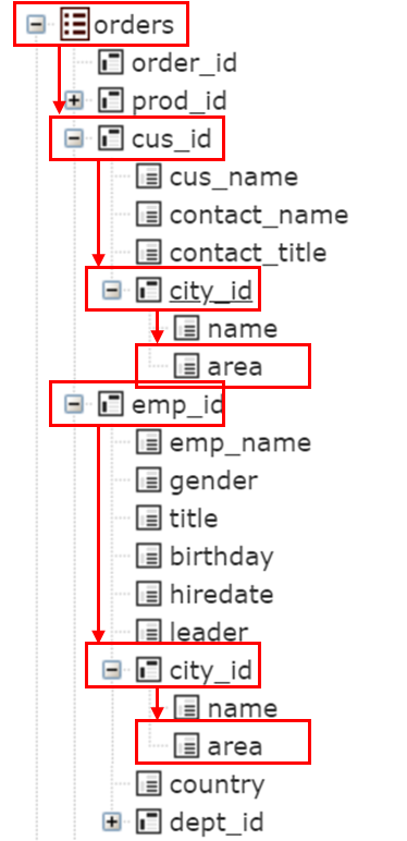
This tree structure expresses multi-layer dimension table associations at multiple levels. Such multidimensional analysis pages are not only easy to develop, but it is easy for ordinary business users to understand. This is where DQL’s effect lies.

To summarize, the purpose of wide table is to solve BI query performance and front-end user operation problems. However, while solving these two problems, wide table also brings problems such as data redundancy and poor flexibility. If SPL and DQL are adopted, the two problems can be solved more effectively. Specifically, SPL's real-time association technology and efficient storage scheme solves the performance problem with better result, without data redundancy and less storage space requirement (compression); The semantic layer built through DQL solves the second problem, making real-time association possible, and has the advantages of higher flexibility (it's no longer limited to on-demand modeling of wide table), easier to implement interface, and wider application range.

SPL+DQL inherits (surpasses) the advantages of wide table while improving its disadvantages. This is what BI should be like.