

Comparison test of Python and SPL in data reading and computing performance
Test environment:
System: CentOS7
Virtual machine: VMWare 15.5.1build-15018445
Memory: 32G
CPU: 4
Data: TPCH 1G
Data reading
There are two types of data sources: text file and database. It should be noted that the data involved in this article is not particularly large in volume and can be fully loaded into memory.
The data is stored in an orderstable and the amount of data is 1.5 million rows.
Text data
The size of text file is 172M. The data row is split by symbol “|”, and presented in the following form:
1|18451|O|193738.97|1996-01-02|5-LOW|Clerk#000000951|0|nstructions sleep furiously among |
2|39001|O|41419.39|1996-12-01|1-URGENT|Clerk#000000880|0| foxes. pending accounts at the pending, silent asymptot|
3|61657|F|208403.57|1993-10-14|5-LOW|Clerk#000000955|0|sly final accounts boost. carefully regular ideas cajole carefully. depos|
4|68389|O|30234.04|1995-10-11|5-LOW|Clerk#000000124|0|sits. slyly regular warthogs cajole. regular, regular theodolites acro|
5|22243|F|149065.30|1994-07-30|5-LOW|Clerk#000000925|0|quickly. bold deposits sleep slyly. packages use slyly|
...
Reading the text file in Python:
import pandas as pd
orders_file="/svmiracle/tpchdata/orders.tbl"
data = pd.read_csv(orders_file,index_col=0,sep="|",header=None)
Time consumed: 7.84 seconds.
Reading the text file in SPL:
A |
|
1 |
'/svmiracle/tpchdata/orders.tbl |
2 |
=file(A1).import(;,"|") |
Time consumed: 6.21 seconds.
SPL has unique binary file format, which can greatly improve the reading efficiency.
After saving the orderstable as a binary file in btx format, its size is 148.5M. SPL reads the binary file:
A |
|
1 |
'/svmiracle/tpchdata/orders.btx |
2 |
=file(A1).import@b() |
Time consumed: 2.56 seconds.
Since Python doesn't provide a common binary file format, we won't compare it here.
SPL can also read the file in parallel:
A |
|
1 |
'/svmiracle/tpchdata/orders.tbl |
2 |
=file(A1).import@m(;,"|") |
Time consumed: 1.68 seconds.
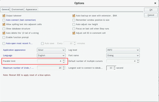
The @moption represents reading data in parallel, which can speed up. However, the order of result set may change, and hence it is recommended to avoid using this option when order is important.
The number of threads for the @moption is set in SPL Tools - Options, as shown in the following figure:
SPL can also read btx file in parallel by adding the same option @m:
A |
|
1 |
'/svmiracle/tpchdata/orders.btx |
2 |
=file(A1).import@mb() |
Time consumed: 0.73 seconds.
Parallel processing of Python itself is fake. Depending on a third-party library to process in parallel will be inconvenient and ineffective, so we won't test Python for its parallel reading ability.
Database
We take the oracle database as an example to test.
Reading the database in Python:
import cx_Oracle
import pandas as pd
pd.set_option('display.max_columns',None)
db = cx_Oracle.connect('kezhao','kezhao','192.168.0.121:1521/ORCLCDB')
cs = db.cursor()
sql = "select * from orders"
orders_cs = cs.execute(sql)
orders_data = orders_cs.fetchall()
columns = ["O_ORDERKEY","O_CUSTKEY","O_ORDERSTATUS","O_TOTALPRICE","O_ORDERDATE","O_ORDERPRIORITY","O_CLERK","O_SHIPPRIORITY","O_COMMENT"]
orders=pd.DataFrame(orders_data,columns=columns)
Time consumed: 18.15 seconds.
Reading the database in SPL:
A |
|
1 |
=connect("oracle19") |
2 |
=A1.query@d("select * from orders") |
Time consumed: 47.41 seconds.
Likewise, SPL can read database in parallel:
A |
B |
|
1 |
>n=4 |
/number of threads |
2 |
fork to(n) |
=connect(“oracle19”) |
3 |
=B2.query@dx(“select * from orders where mod(O_ORDERKEY,?)=?”,n,A2-1) |
|
4 |
=A2.conj() |
Time consumed: 10.78 seconds.
Brief summary
Comparison table of data reading abilities (Unit: second)
Data source |
Python |
SPL (serial reading) |
SPL (parallel reading) |
Text file |
7.84 |
6.21 |
1.68 |
Binary file (btx) |
2.56 |
0.73 |
|
Database |
18.15 |
47.41 |
10.78 |
For the reading of text file, there is little difference between SPL and Python under single-thread condition, but the reading speed can be greatly increased once SPL adopts multi-threaded reading mode. If the text file is saved as binary file (btx) of SPL, the reading performance of SPL can be further greatly improved, far surpassing that of Python.
For the reading of database in single thread, Python has obvious advantages. SPL performs unsatisfactorily due to the low performance of Oracle JDBC (the test uses thin JDBCthat Oracle uses most often. It is said that Oracle also has another kind of interface called ociJ DBCthat performs better, but it is troublesome to configure and it is rarely used, so we didn't test). Fortunately, SPL can make up for this disadvantage by utilizing parallel reading.
Basic operation
In this section, we will test the computing performance of Python and SPL through a few basic operations that can be described in SQL without subquery, such as conventional sum, group, and join. The test data is a text file.
Q1
SQL statement for querying is as follows:
select
l_returnflag,
l_linestatus,
sum(l_quantity) as sum_qty,
sum(l_extendedprice) as sum_base_price,
sum(l_extendedprice * (1 - l_discount)) as sum_disc_price,
sum(l_extendedprice * (1 - l_discount) * (1 + l_tax)) as sum_charge,
avg(l_quantity) as avg_qty,
avg(l_extendedprice) as avg_price,
avg(l_discount) as avg_disc,
count(*) as count_order
from
lineitem
where
l_shipdate <= date '1995-12-01' - interval '90' day(3)
group by
l_returnflag,
l_linestatus
order by
l_returnflag,
l_linestatus;
This is a conventional grouping and aggregating operation with small result set.
Python code:
import time
import pandas as pd
dir = "/svmiracle/tpchtbl1g/"
pd.set_option('display.max_columns',None)
columns =["L_SHIPDATE",
"L_QUANTITY",
"L_EXTENDEDPRICE",
"L_DISCOUNT",
"L_TAX",
"L_RETURNFLAG",
"L_LINESTATUS"]
lineitem_all=pd.read_csv(dir+"lineitem.tbl",usecols=columns,sep="|",
parse_dates=['L_SHIPDATE'],
infer_datetime_format=True)
s = time.time()
date = pd.to_datetime("1995-12-01")-pd.to_timedelta(90,unit="D")
lineitem = lineitem_all[lineitem_all['L_SHIPDATE']<=date].copy()
lineitem['REVENUE'] = lineitem.L_EXTENDEDPRICE*(1-lineitem.L_DISCOUNT)
lineitem['CHARGE'] = lineitem.REVENUE*(lineitem.L_TAX+1)
res = lineitem.groupby(['L_RETURNFLAG', 'L_LINESTATUS']) \
.agg(sum_qty=pd.NamedAgg(column='L_QUANTITY',aggfunc='sum'),\
sum_base_price=pd.NamedAgg(column='L_EXTENDEDPRICE',aggfunc='sum'), \
sum_disc_price = pd.NamedAgg(column='REVENUE', aggfunc='sum'), \
sum_charge = pd.NamedAgg(column='CHARGE', aggfunc='sum'), \
avg_qty = pd.NamedAgg(column='L_QUANTITY', aggfunc='mean'), \
avg_price = pd.NamedAgg(column='L_EXTENDEDPRICE', aggfunc='mean'), \
avg_disc = pd.NamedAgg(column='L_DISCOUNT', aggfunc='mean'), \
count_order = pd.NamedAgg(column='L_SHIPDATE', aggfunc='count')) \
.reset_index()
e = time.time()
print(e-s)
print(res)
Time consumed: 1.84 seconds.
SPL Community Edition:
A |
|
1 |
'/svmiracle/tpchtbl1g/ |
2 |
1995-12-01 |
3 |
=A2-90 |
4 |
=file(A1/"lineitem.tbl").import@t(L_SHIPDATE,L_QUANTITY, L_EXTENDEDPRICE,L_DISCOUNT,L_TAX,L_RETURNFLAG,L_LINESTATUS;,"|") |
5 |
=now() |
6 |
=A4.select(L_SHIPDATE<=A3) |
7 |
=A6.groups(L_RETURNFLAG, L_LINESTATUS; sum(L_QUANTITY):sum_qty, sum(L_EXTENDEDPRICE):sum_base_price, sum(dp=L_EXTENDEDPRICE*(1-L_DISCOUNT)):sum_disc_price, sum(dp*L_TAX)+sum_disc_price:sum_charge, avg(L_QUANTITY):avg_qty, avg(L_EXTENDEDPRICE):avg_price, avg(L_DISCOUNT):avg_disc, count(1):count_order) |
8 |
=interval@ms(A5,now()) |
Time consumed: 2.45 seconds.
SPL Enterprise Edition provides vector-style column-wise computing, which can obtain better performance.
A |
|
1 |
'/svmiracle/tpchtbl1g/ |
2 |
1995-12-01 |
3 |
=A2-90 |
4 |
=file(A1/"lineitem.tbl").import@t(L_SHIPDATE,L_QUANTITY, L_EXTENDEDPRICE,L_DISCOUNT,L_TAX,L_RETURNFLAG,L_LINESTATUS;,"|").i() |
5 |
=now() |
6 |
=A4.cursor().select(L_SHIPDATE<=A3) |
7 |
=A6.derive@o(L_EXTENDEDPRICE*(1-L_DISCOUNT):dp) |
8 |
=A7.groups(L_RETURNFLAG, L_LINESTATUS; sum(L_QUANTITY):sum_qty, sum(L_EXTENDEDPRICE):sum_base_price, sum(dp):sum_disc_price, sum(dp*L_TAX)+sum_disc_price:sum_charge, avg(L_QUANTITY):avg_qty, avg(L_EXTENDEDPRICE):avg_price, avg(L_DISCOUNT):avg_disc, count(1):count_order) |
9 |
=interval@ms(A5,now()) |
Time consumed: 1.30 seconds.
All SPL codes support multi-threaded parallel computing.
Parallel computing of SPL Community Edition:
A |
|
1 |
'/svmiracle/tpchtbl1g/ |
2 |
1995-12-01 |
3 |
=A2-90 |
4 |
=file(A1/"lineitem.tbl").import@mt(L_SHIPDATE,L_QUANTITY, L_EXTENDEDPRICE,L_DISCOUNT,L_TAX,L_RETURNFLAG,L_LINESTATUS;,"|") |
5 |
=now() |
6 |
=A4.select@m(L_SHIPDATE<=A3) |
7 |
=A6.groups@m(L_RETURNFLAG, L_LINESTATUS; sum(L_QUANTITY):sum_qty, sum(L_EXTENDEDPRICE):sum_base_price, sum(dp=L_EXTENDEDPRICE*(1-L_DISCOUNT)):sum_disc_price, sum(dp*L_TAX)+sum_disc_price:sum_charge, avg(L_QUANTITY):avg_qty, avg(L_EXTENDEDPRICE):avg_price, avg(L_DISCOUNT):avg_disc, count(1):count_order) |
8 |
=interval@ms(A5,now()) |
Time consumed: 1.25 seconds.
Column-wise parallel computing of SPL Enterprise Edition:
A |
|
1 |
'/svmiracle/tpchtbl1g/ |
2 |
1995-12-01 |
3 |
=A2-90 |
4 |
=file(A1/"lineitem.tbl").import@tm(L_SHIPDATE,L_QUANTITY, L_EXTENDEDPRICE,L_DISCOUNT,L_TAX,L_RETURNFLAG,L_LINESTATUS;,"|").i() |
5 |
=now() |
6 |
=A4.cursor@m().select@m(L_SHIPDATE<=A3) |
7 |
=A6.derive@om(L_EXTENDEDPRICE*(1-L_DISCOUNT):dp) |
8 |
=A7.groups@m(L_RETURNFLAG, L_LINESTATUS; sum(L_QUANTITY):sum_qty, sum(L_EXTENDEDPRICE):sum_base_price, sum(dp):sum_disc_price, sum(dp*L_TAX)+sum_disc_price:sum_charge, avg(L_QUANTITY):avg_qty, avg(L_EXTENDEDPRICE):avg_price, avg(L_DISCOUNT):avg_disc, count(1):count_order) |
9 |
=interval@ms(A5,now()) |
Time consumed: 0.59 seconds.
Q3
SQL statement for querying is as follows:
select * from (
select
l_orderkey,
sum(l_extendedprice * (1 - l_discount)) as revenue,
o_orderdate,
o_shippriority
from
customer,
orders,
lineitem
where
c_mktsegment = 'BUILDING'
and c_custkey = o_custkey
and l_orderkey = o_orderkey
and o_orderdate < date '1995-03-15'
and l_shipdate > date '1995-03-15'
group by
l_orderkey,
o_orderdate,
o_shippriority
order by
revenue desc,
o_orderdate
) where rownum<=10;
This is a typical primary-sub table association, followed by a grouping and aggregating operation.
Python code:
import time
import pandas as pd
dir = "/svmiracle/tpchtbl1g/"
pd.set_option('display.max_columns',None)
cust_cols = ["C_CUSTKEY","C_MKTSEGMENT"]
cust_all = pd.read_csv(dir+"customer.tbl",usecols=cust_cols,sep="|")
orders_cols = ['O_ORDERKEY','O_CUSTKEY','O_ORDERDATE','O_SHIPPRIORITY']
orders_all = pd.read_csv(dir+"orders.tbl",usecols=orders_cols,sep="|",
parse_dates=['O_ORDERDATE'],
infer_datetime_format=True)
lineitem_cols =['L_ORDERKEY','L_EXTENDEDPRICE','L_DISCOUNT','L_SHIPDATE']
lineitem_all = pd.read_csv(dir+"lineitem.tbl",usecols=lineitem_cols,sep="|",
parse_dates=['L_SHIPDATE'],
infer_datetime_format=True)
s = time.time()
date = pd.to_datetime("1995-3-15")
segment = "BUILDING"
cust = cust_all[cust_all['C_MKTSEGMENT']==segment]
orders = orders_all[orders_all['O_ORDERDATE']lineitem = lineitem_all[lineitem_all['L_SHIPDATE']>date].copy()
orders_c = pd.merge(orders,cust,\
left_on='O_CUSTKEY',\
right_on='C_CUSTKEY',\
how='inner')
lineitem['REVENUE'] = lineitem.L_EXTENDEDPRICE*(1-lineitem.L_DISCOUNT)
lineitem_s = lineitem.groupby('L_ORDERKEY').REVENUE.sum()
lineitem_g = pd.DataFrame(lineitem_s,columns=['REVENUE']).reset_index()
orders_cl = pd.merge(orders_c,lineitem_g,\
left_on='O_ORDERKEY',\
right_on='L_ORDERKEY',\
how='inner')
orders_cl.sort_values(by=['REVENUE','O_ORDERDATE'],\
ascending=[False,True],\
ignore_index=True,\
inplace=True)
res = orders_cl[:10][['L_ORDERKEY','REVENUE','O_ORDERDATE','O_SHIPPRIORITY']]
e = time.time()
print(e-s)
print(res)
Time consumed: 1.48 seconds.
SPL Community Edition:
A |
|
1 |
'/svmiracle/tpchtbl1g/ |
2 |
1995-3-15 |
3 |
BUILDING |
4 |
=file(A1/"customer.tbl").import@t(C_CUSTKEY,C_MKTSEGMENT ;,"|") |
5 |
=file(A1/"orders.tbl").import@t(O_ORDERKEY,O_CUSTKEY,O_ORDERDATE,O_SHIPPRIORITY;,"|") |
6 |
=file(A1/"lineitem.tbl").import@t(L_ORDERKEY,L_EXTENDEDPRICE,L_DISCOUNT,L_SHIPDATE;,"|") |
7 |
=now() |
8 |
=A4.select(C_MKTSEGMENT==A3).derive@o().keys@i(C_CUSTKEY) |
9 |
=A5.select(O_ORDERDATE |
10 |
=A6.select(L_SHIPDATE>A2).switch@i(L_ORDERKEY,A9) |
11 |
=A10.groups(L_ORDERKEY.O_ORDERKEY:L_ORDERKEY;sum(L_EXTENDEDPRICE*(1-L_DISCOUNT)):REVENUE,L_ORDERKEY.O_ORDERDATE,L_ORDERKEY.O_SHIPPRIORITY) |
12 |
=A11.top(10;-REVENUE,O_ORDERDATE) |
13 |
=interval@ms(A7,now()) |
Time consumed: 1.87 seconds.
Column-wise computing of SPL Enterprise Edition:
A |
|
1 |
'/svmiracle/tpchtbl1g/ |
2 |
1995-3-15 |
3 |
BUILDING |
4 |
=file(A1/"customer.tbl").import@t(C_CUSTKEY,C_MKTSEGMENT ;,"|").i() |
5 |
=file(A1/"orders.tbl").import@t(O_ORDERKEY,O_CUSTKEY,O_ORDERDATE,O_SHIPPRIORITY;,"|").i() |
6 |
=file(A1/"lineitem.tbl").import@t(L_ORDERKEY,L_EXTENDEDPRICE,L_DISCOUNT,L_SHIPDATE;,"|").i() |
7 |
=now() |
8 |
=A4.select@v(C_MKTSEGMENT==A3).(C_CUSTKEY) |
9 |
=A5.select@v(O_ORDERDATE |
10 |
=A6.select@v(L_SHIPDATE>A2).join@i(L_ORDERKEY,A9,O_ORDERDATE,O_SHIPPRIORITY) |
11 |
=A10.groups(L_ORDERKEY;sum(L_EXTENDEDPRICE*(1-L_DISCOUNT)):REVENUE,O_ORDERDATE,O_SHIPPRIORITY) |
12 |
=A11.top(10;-REVENUE,O_ORDERDATE) |
13 |
=interval@ms(A7,now()) |
Time consumed: 0.71 seconds.
Let's see the performance of SPL's multi-threaded parallel computing:
Parallel computing of SPL Community Edition:
A |
|
1 |
'/svmiracle/tpchtbl1g/ |
2 |
1995-3-15 |
3 |
BUILDING |
4 |
=file(A1/"customer.tbl").import@mt(C_CUSTKEY,C_MKTSEGMENT ;,"|") |
5 |
=file(A1/"orders.tbl").import@mt(O_ORDERKEY,O_CUSTKEY,O_ORDERDATE,O_SHIPPRIORITY;,"|") |
6 |
=file(A1/"lineitem.tbl").import@mt(L_ORDERKEY,L_EXTENDEDPRICE,L_DISCOUNT,L_SHIPDATE;,"|") |
7 |
=now() |
8 |
=A4.select@m(C_MKTSEGMENT==A3).derive@o().keys@i(C_CUSTKEY) |
9 |
=A5.select@m(O_ORDERDATE |
10 |
=A6.select@m(L_SHIPDATE>A2).switch@i(L_ORDERKEY,A9) |
11 |
=A10.groups@m(L_ORDERKEY.O_ORDERKEY:L_ORDERKEY;sum(L_EXTENDEDPRICE*(1-L_DISCOUNT)):REVENUE,L_ORDERKEY.O_ORDERDATE,L_ORDERKEY.O_SHIPPRIORITY) |
12 |
=A11.top(10;-REVENUE,O_ORDERDATE) |
13 |
=interval@ms(A7,now()) |
Time consumed: 1.16 seconds.
Column-wise parallel computing of SPL Enterprise Edition:
A |
|
1 |
'/svmiracle/tpchtbl1g/ |
2 |
1995-3-15 |
3 |
BUILDING |
4 |
=file(A1/"customer.tbl").import@mt(C_CUSTKEY,C_MKTSEGMENT ;,"|").i() |
5 |
=file(A1/"orders.tbl").import@mt(O_ORDERKEY,O_CUSTKEY,O_ORDERDATE,O_SHIPPRIORITY;,"|").i() |
6 |
=file(A1/"lineitem.tbl").import@mt(L_ORDERKEY,L_EXTENDEDPRICE,L_DISCOUNT,L_SHIPDATE;,"|").i() |
7 |
=now() |
8 |
=A4.select@vm(C_MKTSEGMENT==A3).(C_CUSTKEY) |
9 |
=A5.select@mv(O_ORDERDATE |
10 |
=A6.select@mv(L_SHIPDATE>A2).join@i(L_ORDERKEY,A9,O_ORDERDATE,O_SHIPPRIORITY) |
11 |
=A10.groups@m(L_ORDERKEY;sum(L_EXTENDEDPRICE*(1-L_DISCOUNT)):REVENUE,O_ORDERDATE,O_SHIPPRIORITY) |
12 |
=A11.top(10;-REVENUE,O_ORDERDATE) |
13 |
=interval@ms(A7,now()) |
Time consumed: 0.51 seconds.
Q6
SQL statement for querying is as follows:
select
sum(l_extendedprice * l_discount) as revenue
from
lineitem
where
l_shipdate >= date '1995-01-01'
and l_shipdate < date '1995-01-01' + interval '1' year
and l_discount between 0.05 - 0.01 and 0.05 + 0.01
and l_quantity < 24;
This is a simple filtering and aggregation operation on a single table.
Python code:
import time
import pandas as pd
dir = "/svmiracle/tpchtbl1g/"
pd.set_option('display.max_columns',None)
lineitem_cols =['L_SHIPDATE','L_QUANTITY','L_EXTENDEDPRICE','L_DISCOUNT']
lineitem_all = pd.read_csv(dir+"lineitem.tbl",usecols=lineitem_cols,sep="|",
parse_dates=['L_SHIPDATE'],
infer_datetime_format=True)
s = time.time()
date_s = pd.to_datetime("1995-01-01")
date_e = date_s+pd.DateOffset(years=1)
mi = 0.05 - 0.01
ma = 0.05 + 0.01
qt = 24
lineitem = lineitem_all[(lineitem_all['L_SHIPDATE'].between(date_s,date_e,"left"))& \
(lineitem_all['L_DISCOUNT'].between(mi,ma,"both"))& \
(lineitem_all['L_QUANTITY']res = (lineitem.L_EXTENDEDPRICE * lineitem.L_DISCOUNT).sum()
e = time.time()
print(e-s)
print(res)
Time consumed: 0.19 seconds.
SPL Community Edition:
A |
|
1 |
'/svmiracle/tpchtbl1g/ |
2 |
1995-01-01 |
3 |
=elapse@y(A2,1) |
4 |
=0.05 - 0.01 |
5 |
=0.05 + 0.01 |
6 |
24 |
7 |
=file(A1/"lineitem.tbl").import@t(L_SHIPDATE,L_QUANTITY,L_EXTENDEDPRICE,L_DISCOUNT;,"|") |
8 |
=now() |
9 |
=A7.select(L_DISCOUNT>=A4&&L_DISCOUNT=A2&&L_SHIPDATE |
10 |
=A9.sum(L_EXTENDEDPRICE*L_DISCOUNT) |
11 |
=interval@ms(A8,now()) |
Time consumed: 1.54 seconds.
Column-wise computing of SPL Enterprise Edition:
A |
|
1 |
'/svmiracle/tpchtbl1g/ |
2 |
1995-01-01 |
3 |
=elapse@y(A2,1) |
4 |
=0.05 - 0.01 |
5 |
=0.05 + 0.01 |
6 |
24 |
7 |
=file(A1/"lineitem.tbl").import@t(L_SHIPDATE,L_QUANTITY,L_EXTENDEDPRICE,L_DISCOUNT;,"|").i() |
8 |
=now() |
9 |
=A7.sum(if(L_DISCOUNT>=A4&&L_DISCOUNT=A2&&L_SHIPDATE |
10 |
=interval@ms(A8,now()) |
Time consumed: 0.55 seconds
Let's see the performance of SPL's multi-threaded parallel computing:
Parallel computing of SPL Community Edition:
A |
|
1 |
'/svmiracle/tpchtbl1g/ |
2 |
1995-01-01 |
3 |
=elapse@y(A2,1) |
4 |
=0.05 - 0.01 |
5 |
=0.05 + 0.01 |
6 |
24 |
7 |
=file(A1/"lineitem.tbl").import@mt(L_SHIPDATE,L_QUANTITY,L_EXTENDEDPRICE,L_DISCOUNT;,"|") |
8 |
=now() |
9 |
=A7.select@m(L_DISCOUNT>=A4&&L_DISCOUNT=A2&&L_SHIPDATE |
10 |
=A9.sum(L_EXTENDEDPRICE*L_DISCOUNT) |
11 |
=interval@ms(A8,now()) |
Time consumed: 0.55 seconds.
Column-wise parallel computing of SPL Enterprise Edition:
A |
|
1 |
'/svmiracle/tpchtbl1g/ |
2 |
1995-01-01 |
3 |
=elapse@y(A2,1) |
4 |
=0.05 - 0.01 |
5 |
=0.05 + 0.01 |
6 |
24 |
7 |
=file(A1/"lineitem.tbl").import@t(L_SHIPDATE,L_QUANTITY,L_EXTENDEDPRICE,L_DISCOUNT;,"|").i() |
8 |
=now() |
9 |
=A7.groups@m(;sum(if(L_DISCOUNT>=A4&&L_DISCOUNT=A2&&L_SHIPDATE |
10 |
=interval@ms(A8,now()) |
Time consumed: 0.22 seconds
Brief summary
Performance comparison between Python and SPL on basic SQL-style calculation:
Q1 |
Q3 |
Q6 |
|
Python |
1.84 |
1.48 |
0.19 |
SPL Community Edition |
2.45 |
1.87 |
1.54 |
SPL Enterprise Edition |
1.30 |
0.71 |
0.55 |
SPL Community Edition (parallel computing) |
1.25 |
1.16 |
0.55 |
SPL Enterprise Edition (parallel computing) |
0.59 |
0.51 |
0.22 |
For these basic operations, Python performs better than SPL Community Edition. The reason is that SPL uses object sequence in order to support generic data, which requires more judgements during calculation, while the columns in Python's DataFrame are all of a single data type, and hence Python has faster computing speed. SPL Enterprise Edition provides pure table sequence with a single column data type similar to the data structure of Python, and the performance is usually better than that of Python. After adopting the parallel computing, the computing abilities of both Community Edition and Enterprise Edition are improved. Q6 is the simplest operation involving the filtering, multiplication and summation, which are exactly what Pandas' matrix data structure does best, so the computing performance of Pandas is particularly good, surpassing that of parallel computing of SPL Enterprise Edition.
Non-basic operation
Now let's seeanother two operations that cannot be described in SQL unless nesting subqueries, as well as one operation where data characteristics can be utilized to improve performance.
Q2
SQL statement for querying is as follows:
select * from (
select
s_acctbal,s_name,n_name,p_partkey,p_mfgr,s_address,s_phone,s_comment
from part,supplier,partsupp,nation,region
where
p_partkey = ps_partkey
and s_suppkey = ps_suppkey
and p_size = 25
and p_type like '%COPPER'
and s_nationkey = n_nationkey
and n_regionkey = r_regionkey
and r_name = 'ASIA'
and ps_supplycost = (
select
min(ps_supplycost)
from
partsupp,
supplier,
nation,
region
where
p_partkey = ps_partkey
and s_suppkey = ps_suppkey
and s_nationkey = n_nationkey
and n_regionkey = r_regionkey
and r_name = 'ASIA'
)
order by
s_acctbal desc,n_name,s_name,p_partkey
)
where rownum <= 100;
This SQL statement includes not only basic operations like association and aggregation, but the operation of taking all minimum value records.
Python code:
import time
import pandas as pd
pd.set_option('display.max_columns',None)
dir = "/svmiracle/tpchtbl1g/"
size=25
type="COPPER"
name="ASIA"
def min_r(df):
mi = df['PS_SUPPLYCOST'].min()
minr = df[df['PS_SUPPLYCOST']==mi]
return minr
region_all = pd.read_csv(dir+"region.tbl",
usecols=['R_NAME','R_REGIONKEY'],sep='|')
nation_all = pd.read_csv(dir+"nation.tbl",
usecols=['N_NATIONKEY','N_REGIONKEY','N_NAME'],sep='|')
part_all = pd.read_csv(dir+"part.tbl",
usecols=['P_PARTKEY','P_MFGR','P_SIZE','P_TYPE'],sep='|')
supplier_all = pd.read_csv(dir+"supplier.tbl",
usecols=['S_SUPPKEY','S_NAME','S_ADDRESS','S_NATIONKEY','S_PHONE','S_ACCTBAL','S_COMMENT'],sep='|')
partsupp_all = pd.read_csv(dir+"partsupp.tbl",
usecols=['PS_PARTKEY','PS_SUPPKEY','PS_SUPPLYCOST'],sep='|')
s = time.time()
for i in range(len(region_all)):
sr = region_all.iloc[i]
if sr.R_NAME==name:
rg = sr.R_REGIONKEY
break
nation = nation_all[nation_all['N_REGIONKEY']==rg]
part = part_all[(part_all['P_SIZE']==size)& (part_all['P_TYPE'].str.contains(type))]
sup_nat = pd.merge(supplier_all,nation,\
left_on='S_NATIONKEY',right_on='N_NATIONKEY',how='inner')
ps_par = pd.merge(partsupp_all,part,\
left_on='PS_PARTKEY',right_on='P_PARTKEY',how='inner')
ps_par_sup_nat = pd.merge(ps_par,sup_nat,\
left_on='PS_SUPPKEY',right_on='S_SUPPKEY',how='inner')
ps_min = ps_par_sup_nat.groupby('PS_PARTKEY').apply(lambda x:min_r(x))
ps_min_100 = ps_min.sort_values(['S_ACCTBAL','N_NAME','S_NAME','P_PARTKEY'],ascending=[False,True,True,True]).iloc[:100]
res = ps_min_100[['S_ACCTBAL','S_NAME','N_NAME','P_PARTKEY','P_MFGR','S_ADDRESS','S_PHONE','S_COMMENT']]
e = time.time()
print(e-s)
print(res)
It takes 1.23 seconds, which are mainly spent on searching for the minimum value records of each group.
SPL Community Edition:
A |
|
1 |
'/svmiracle/tpchtbl1g/ |
2 |
>size=25 |
3 |
>type="COPPER" |
4 |
>name="ASIA" |
5 |
=file(A1/"region.tbl").import@t(R_NAME,R_REGIONKEY;,"|") |
6 |
=file(A1/"nation.tbl").import@t(N_NATIONKEY,N_REGIONKEY,N_NAME;,"|") |
7 |
=file(A1/"part.tbl").import@t(P_PARTKEY,P_MFGR,P_SIZE,P_TYPE;,"|") |
8 |
=file(A1/"supplier.tbl").import@t(S_SUPPKEY,S_NAME,S_ADDRESS,S_NATIONKEY,S_PHONE,S_ACCTBAL,S_COMMENT;,"|") |
9 |
=file(A1/"partsupp.tbl").import@t(PS_PARTKEY,PS_SUPPKEY,PS_SUPPLYCOST;,"|") |
10 |
=now() |
11 |
=A5.select@1(R_NAME==name).R_REGIONKEY |
12 |
=A6.select(N_REGIONKEY==A11).derive@o().keys@i(N_NATIONKEY) |
13 |
=A7.select(P_SIZE==size && pos@t(P_TYPE,type)).derive@o().keys@i(P_PARTKEY) |
14 |
=A8.switch@i(S_NATIONKEY,A12).keys@i(S_SUPPKEY) |
15 |
=A9.switch@i(PS_PARTKEY,A13;PS_SUPPKEY,A14) |
16 |
=A15.groups(PS_PARTKEY;minp@a(PS_SUPPLYCOST)).conj(#2) |
17 |
=A16.top(100;-PS_SUPPKEY.S_ACCTBAL,PS_SUPPKEY.S_NATIONKEY.N_NAME,PS_SUPPKEY.S_NAME,PS_PARTKEY.P_PARTKEY) |
18 |
=A17.new(PS_SUPPKEY.S_ACCTBAL,PS_SUPPKEY.S_NAME,PS_SUPPKEY.S_NATIONKEY.N_NAME,PS_PARTKEY.P_PARTKEY,PS_PARTKEY.P_MFGR,PS_SUPPKEY.S_ADDRESS,PS_SUPPKEY.S_PHONE,PS_SUPPKEY.S_COMMENT) |
19 |
=interval@ms(A10,now()) |
Time consumed: 0.10 seconds
SPL regards searching for the minimum value record as an aggregation function similar to sumand count, so groups(…;minp@())is written directly in A16to calculate result in one go, the performance is thus better.
Column-wise computing of SPL Enterprise Edition:
A |
|
1 |
'/svmiracle/tpchtbl1g/ |
2 |
>size=25 |
3 |
>type="COPPER" |
4 |
>name="ASIA" |
5 |
=file(A1/"region.tbl").import@t(R_NAME,R_REGIONKEY;,"|").i() |
6 |
=file(A1/"nation.tbl").import@t(N_NATIONKEY,N_REGIONKEY,N_NAME;,"|").i() |
7 |
=file(A1/"part.tbl").import@t(P_PARTKEY,P_MFGR,P_SIZE,P_TYPE;,"|").i() |
8 |
=file(A1/"supplier.tbl").import@t(S_SUPPKEY,S_NAME,S_ADDRESS,S_NATIONKEY,S_PHONE,S_ACCTBAL,S_COMMENT;,"|").i() |
9 |
=file(A1/"partsupp.tbl").import@t(PS_PARTKEY,PS_SUPPKEY,PS_SUPPLYCOST;,"|").i() |
10 |
=now() |
11 |
=A5.select@v1(R_NAME==name).R_REGIONKEY |
12 |
=A6.select@v(N_REGIONKEY==A11).derive@o().keys@i(N_NATIONKEY) |
13 |
=A7.select@v(P_SIZE==size && pos@t(P_TYPE,type)).derive@o().keys@i(P_PARTKEY) |
14 |
=A8.switch@i(S_NATIONKEY,A12).keys@i(S_SUPPKEY) |
15 |
=A9.switch@i(PS_PARTKEY,A13;PS_SUPPKEY,A14) |
16 |
=A15.groups(PS_PARTKEY;minp@a(PS_SUPPLYCOST)).conj(#2) |
17 |
=A16.top(100;-PS_SUPPKEY.S_ACCTBAL,PS_SUPPKEY.S_NATIONKEY.N_NAME,PS_SUPPKEY.S_NAME,PS_PARTKEY.P_PARTKEY) |
18 |
=A17.new(PS_SUPPKEY.S_ACCTBAL,PS_SUPPKEY.S_NAME,PS_SUPPKEY.S_NATIONKEY.N_NAME,PS_PARTKEY.P_PARTKEY,PS_PARTKEY.P_MFGR,PS_SUPPKEY.S_ADDRESS,PS_SUPPKEY.S_PHONE,PS_SUPPKEY.S_COMMENT) |
19 |
=interval@ms(A10,now()) |
Time consumed: 0.05 seconds.
Q13
SQL statement for querying is as follows:
select
c_count,
count(*) as custdist
from (
select
c_custkey,
count(o_orderkey) c_count
from
customer left outer join orders on
c_custkey = o_custkey
and o_comment not like '%special%accounts%'
group by
c_custkey
) c_orders
group by
c_count
order by
custdist desc,
c_count desc;
To put it simply, this query is to perform two rounds of conventional grouping on the orders table. The first round is to group by custkey and calculate the number of orders placed by each customer, and the second round is to group by the number of orders and calculate the number of customers corresponding to each number of orders. In this statement, the string-matching operation is involved.
Python code:
import time
import pandas as pd
pd.set_option('display.max_columns',None)
dir = "/svmiracle/tpchtbl1g/"
filter=".*special.*accounts.*"
orders_all = pd.read_csv(dir+"orders.tbl",
usecols=['O_CUSTKEY','O_COMMENT'],sep='|')
s = time.time()
orders = orders_all[~(orders_all['O_COMMENT'].str.match(filter))]
orders_cnt = orders.groupby('O_CUSTKEY').size()
len_orders_cnt = len(orders_cnt)
orders_cnt_cnt = orders_cnt.groupby(orders_cnt).size()
with open(dir+"customer.tbl",'rb') as f:
n_row = -1
for i in f:
n_row+=1
num = n_row - len_orders_cnt
orders_cnt_cnt[0] = num
res_df = pd.DataFrame(orders_cnt_cnt).reset_index(drop=False)\
.rename(columns={'index':'c_count',0:'custdist'})
res = res_df.sort_values(by=['custdist','c_count'],ascending=False).reset_index()
e = time.time()
print(e-s)
print(res)
It takes 2.26 seconds, most of which are spent on matching strings.
SPL Community Edition:
A |
|
1 |
'/svmiracle/tpchtbl1g/ |
2 |
>filter="*special*accounts*" |
3 |
=file(A1/"orders.tbl").import@t(O_CUSTKEY,O_COMMENT;,"|") |
4 |
=file(A1/"customer.tbl").cursor@t() |
5 |
=now() |
6 |
=A3.select(!like(O_COMMENT,filter)) |
7 |
=A4.skip() |
8 |
=A6.groups@u(O_CUSTKEY;count(1):c_count) |
9 |
=A8.len() |
10 |
=A8.groups@u(c_count;count(1):custdist) |
11 |
=A10.insert(0,0,A7-A9) |
12 |
=A10.sort@z(custdist,c_count) |
13 |
=interval@ms(A5,now()) |
Time consumed: 1.99 seconds
Column-wise computing of SPL Enterprise Edition:
A |
|
1 |
'/svmiracle/tpchtbl1g/ |
2 |
>filter="*special*accounts*" |
3 |
=file(A1/"orders.tbl").import@t(O_CUSTKEY,O_COMMENT;,"|").i() |
4 |
=file(A1/"customer.tbl").cursor@t() |
5 |
=now() |
6 |
=A3.select@v(!like(O_COMMENT,filter)) |
7 |
=A4.skip() |
8 |
=A6.groups@u(O_CUSTKEY;count(1):c_count) |
9 |
=A8.len() |
10 |
=A8.groups@u(c_count;count(1):custdist) |
11 |
=new(0:c_count,A7-A9:custdist).i() |
12 |
=A10|A11 |
13 |
=A12.sort@zv(custdist,c_count) |
14 |
=interval@ms(A5,now()) |
Time consumed: 0.58 seconds
Q3 (ordered computing)
Since Python doesn’t support order-related operations, Python code is not provided.
In contrast, SPL can utilize the characteristic of data orderliness, the running speed is thus further improved. For example, in this example, we assume that the customer.tblis ordered by C_CUSTKEY, the orderstable is ordered by O_ORDERKEY, and the lineitem.tblis ordered by L_ORDERKEY, let's see the performance of SPL’s ordered column-wise computing.
SPL Community Edition (ordered computing):
A |
|
1 |
'/svmiracle/tpchtbl1g/ |
2 |
1995-3-15 |
3 |
BUILDING |
4 |
=file(A1/"customer_s.tbl").import@t(C_CUSTKEY,C_MKTSEGMENT ;,"|") |
5 |
=file(A1/"orders_s.tbl").import@t(O_ORDERKEY,O_CUSTKEY,O_ORDERDATE,O_SHIPPRIORITY;,"|") |
6 |
=file(A1/"lineitem_s.tbl").import@t(L_ORDERKEY,L_EXTENDEDPRICE,L_DISCOUNT,L_SHIPDATE;,"|") |
7 |
=now() |
8 |
=A4.select(C_MKTSEGMENT==A3).derive@o().keys@i(C_CUSTKEY) |
9 |
=A5.select(O_ORDERDATE |
10 |
=A6.select(L_SHIPDATE>A2).join@mi(L_ORDERKEY,A9,O_ORDERDATE,O_SHIPPRIORITY) |
11 |
=A10.groups(L_ORDERKEY;sum(L_EXTENDEDPRICE*(1-L_DISCOUNT)):REVENUE,O_ORDERDATE,O_SHIPPRIORITY) |
12 |
=A11.top(10;-REVENUE,O_ORDERDATE) |
13 |
=interval@ms(A7,now()) |
Time consumed: 1.52 seconds
SPL Enterprise Edition (ordered column-wise computing):
A |
|
1 |
'/svmiracle/tpchtbl1g/ |
2 |
1995-3-15 |
3 |
BUILDING |
4 |
=file(A1/"customer_s.tbl").import@t(C_CUSTKEY,C_MKTSEGMENT ;,"|").i() |
5 |
=file(A1/"orders_s.tbl").import@t(O_ORDERKEY,O_CUSTKEY,O_ORDERDATE,O_SHIPPRIORITY;,"|").i() |
6 |
=file(A1/"lineitem_s.tbl").import@t(L_ORDERKEY,L_EXTENDEDPRICE,L_DISCOUNT,L_SHIPDATE;,"|").i() |
7 |
=now() |
8 |
=A4.select@v(C_MKTSEGMENT==A3).(C_CUSTKEY) |
9 |
=A5.select@v(O_ORDERDATE |
10 |
=A6.select@v(L_SHIPDATE>A2).join@mi(L_ORDERKEY,A9,O_ORDERDATE,O_SHIPPRIORITY) |
11 |
=A10.groups(L_ORDERKEY;sum(L_EXTENDEDPRICE*(1-L_DISCOUNT)):REVENUE,O_ORDERDATE,O_SHIPPRIORITY) |
12 |
=A11.top(10;-REVENUE,O_ORDERDATE) |
13 |
=interval@ms(A7,now()) |
Time consumed: 0.43 seconds
Because the data is in order, the join@moption can be used to implement merge and association during association to reduce the cost of association.
Brief summary
Taking all minimum value records after grouping in Q2, matching strings in Q13, and ordered associating in Q3 are all the non-basic operation. The following table is the performance comparison result between Python and SPL.
Q2 |
Q13 |
Q3 (ordered computing) |
|
Python |
1.23 |
2.26 |
1.48 |
SPL (row-wise computing) |
0.10 |
1.99 |
1.52 |
SPL (column-wise computing) |
0.05 |
0.58 |
0.43 |
Since Python can't make use of the characteristic of data orderliness, the code remains unchanged, and hence the time filled in this table is that consumed in Q3.
Python is deficient in terms of non-basic operation. Due to the lack of the computing methods in this regard, it has to adopt indirect or conventional method, resulting in much worse performance than SPL.
Summary
1. Data reading ability
When reading text file, there is little difference between Python and SPL, and SPL is slightly stronger. SPL has a unique binary file format btx, and its reading efficiency is much higher than that of Python; in terms of reading database, SPL is at a clear disadvantage due to the negative effectof JDBC.
SPL supports reading data in parallel, which can speed up a lot when data order is not regarded as important, expand the advantage of reading text file, and make up for its disadvantage of reading database.
2. Basic operation
Python relies on Pandas to perform calculation. Since the structured data structure of Pandas is DataFrame, which is essentially a matrix, it has the advantages of matrix calculation when facing basic operations (sum, group, join, etc.). Under single-thread condition, Python performs better than SPL row-wise computing, but not as well as SPL column-wise computing. If the multi-thread computing ability of SPL is taken into account, SPL is better than Python as a whole.
3. Non-basic operation
In terms of non-basic operation, the matrix data structure of Pandas becomes a disadvantage. For example, matching strings in Q13 is not what matrix is good at since the matrix is originally used to calculate numbers, so the performance of Pandas in Q13 is not good; Another disadvantage of Pandas is that its operation ability is incomplete. For example, searching for all minimum value records after grouping in Q2, Pandas has to calculate the minimum value first, and then select all minimum value records, so it needs to transverse one more time, which will naturally lose performance. In addition, Python cannot utilize the characteristic of data orderliness. In contrast, SPL can utilize the orderliness to improve performance, for example, SPL uses join@m()for the ordered association in Q3, converting complex jointo mergeandjoin, the amount of calculation is naturally much lower.
SPL Official Website 👉 http://www.scudata.com
SPL Feedback and Help 👉 https://www.reddit.com/r/esProc
SPL Learning Material 👉 http://c.scudata.com
SPL Source Code and Package 👉 https://github.com/SPLWare/esProc
Discord 👉 https://discord.gg/ydhVnFH9
Youtube 👉 https://www.youtube.com/@esProc_SPL


Chinese version