

How to perform mixed computing with multiple data sources
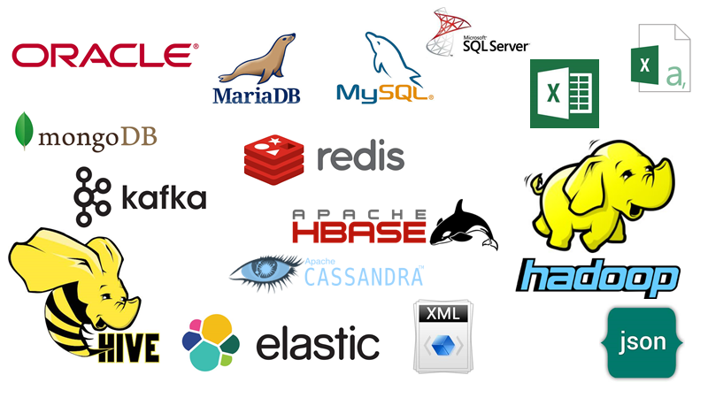
Early applications usually only connected to one database, and calculations were also performed in the database, with little or no problem of mixed calculations from multiple data sources. The data sources of modern applications have become very rich, and the same application may also access multiple data sources, such as various SQL and NoSQL databases, text/XLS, WebService/Restful, Kafka, Hadoop…. Mixed computing on multiple data sources is an unavoidable problem that needs to be addressed.
Direct hard coding to implement in applications is very cumbersome, and commonly used application development languages such as Java are not good at doing such things. Compared to SQL, their simplicity is far inferior.
It is also not appropriate to import multi-source data into one database and then calculate. Not to mention that importing takes time and results in a loss of data real-timeness, the importing of certain data (such as data supported by Mongodb and multi-layer document data) into a relational database losslessly is a very difficult and costly task. After all, the existence of these diverse data sources has a reason and cannot be easily replaced by relational databases. Otherwise, there’s no need to invent Mongodb, just use MySQL.
What about a logical data warehouse? It sounds very heavy. Before use, it is necessary to define metadata to map these diverse data sources, which is very cumbersome. Moreover, most logical data warehouses are still SQL based, making it difficult to map these diverse data losslessly.
What about the pile of computing frameworks? Especially the stream computing framework. It is possible to access many data sources, but the computing itself provides very little functionality. Either use SQL, there will be mapping difficulties like a logical data warehouse; To freely access various data sources, you have to write your own calculation code in Java.
Facing mixed computing problems on multiple data sources, esProc SPL is a good approach.
esProc SPL is an open source computing engine developed purely in Java, and it is here https://github.com/SPLWare/esProc .
How can esProc SPL solve this problem? There are mainly two aspects:
-
The abstract access interface for diverse data sources can map a wide range of data into a few data objects.
-
Based on the data objects in 1, independently implement sufficiently rich computing power independent of the data source.
With these two abilities, when encountering new data sources, just encapsulate the interface and constantly supplement it.
esProc SPL provides two basic data objects: table sequence and cursor, corresponding to in-memory data table and streaming data table, respectively.
Almost all data sources, including relational databases, provide interfaces to return these two types of data objects: small data is read at one time, and an in-memory data table (table sequence) is used; Big data needs to be gradually returned using a streaming data table (cursor). With these two types of data objects, almost all data sources can be covered.
In this way, there is no need to define metadata for mapping in advance, and the data can be accessed directly using the methods provided by the data source itself, and then encapsulated into one of these two types of data objects. This can preserve the characteristics of the data source and fully utilize its storage and computing capabilities. Of course, there is no need to perform a “certain” import action on the data first, and real-time access can be implemented. These two types of data objects share the common capabilities of diverse data source access interfaces, while the mapping data table method used in a logical data warehouse does not correctly abstract the common characteristics of diverse data sources, and its applicability is much narrower.
It should be noted that SPL’s table sequence and cursor both support multi-layer structured data as well as text data, which allows for the receiving and processing of JSON data (or its binary variant).
Take a look at some examples:
Relational database, A2 returns a table sequence, A3 returns a cursor
| A | |
|---|---|
| 1 | =connect("MyCompany") |
| 2 | =A1.query("select * from employees order by hire_date asc limit 100") |
| 3 | =A1.cursor("select * from salaries") |
| 4 | >A1.close() |
Local file, A1/A3 returns a table sequence, A2 returns a cursor
| A | |
|---|---|
| 1 | =T("Orders.csv") |
| 2 | =file("sales.txt").cursor@t() |
| 3 | =file("Orders.xls").xlsimport@t() |
Restful, A1 returns text in JSON format
| A | |
|---|---|
| 1 | =httpfile("http://127.0.0.1:6868/restful/emp_orders").read() |
| 2 | =json(A1) |
Elastic Search
| A | |
|---|---|
| 1 | >apikey="Authorization:ApiKey a2x6aEF……KZ29rT2hoQQ==" |
| 2 | '{ "counter" : 1, "tags" : ["red"] ,"beginTime":"2022-01-03" ,"endTime":"2022-02-15" } |
| 3 | =es_rest("https://localhost:9200/index1/_doc/1", "PUT",A2;"Content-Type: application/x-ndjson",apikey) |
Mongodb, A2 returns a table sequence, A3 returns a cursor
| A | |
|---|---|
| 1 | =mongo_open("mongodb://127.0.0.1:27017/mymongo") |
| 2 | =mongo_shell(A1,"{'find':'orders',filter:{OrderID: {$gte: 50}},batchSize:100}") |
| 3 | =mongo_shell@dc(A1,"{'find':'orders',filter:{OrderID: { $gte: 50}},batchSize:10}") |
| 4 | =mongo_close(A1) |
Kafka, A2 returns a table sequence containing JSON data, A3 returns a cursor
| A | |
|---|---|
| 1 | =kafka_open("/kafka/my.properties", "topic1") |
| 2 | =kafka_poll(A1) |
| 3 | =kafka_poll@c(A1) |
| 4 | =kafka_close(A1) |
HBase, A2/A3 returns a tables equence, A4 returns a cursor
| A | |
|---|---|
| 1 | =hbase_open("hdfs://192.168.0.8", "192.168.0.8") |
| 2 | =hbase_get(A1,"Orders","row1","datas:Amount":number:amt,"datas:OrderDate":date:od) |
| 3 | =hbase_scan(A1,"Orders") |
| 4 | =hbase_scan@c(A1,"Orders") |
| 5 | =hbase_close(A1) |
There are already many data sources encapsulated in esProc SPL and they are still increasing:
esProc SPL provides comprehensive computing power for table sequences, including filtering, grouping, sorting, join, etc. Its richness far exceeds that of SQL, and most operations can be implemented in just one line:
Filter:T.select(Amount>1000 && Amount<=3000 && like(Client,"*s*"))
Sort:T.sort(Client,-Amount)
Distinct:T.id(Client)
Group:T.groups(year(OrderDate);sum(Amount))
Join:join(T1:O,SellerId; T2:E,EId)
TopN:T.top(-3;Amount)
TopN in group:T.groups(Client;top(3,Amount))
There are similar calculations on cursors, and the syntax is almost identical. We won’t provide detailed examples here. Interested friends can refer to the materials on the esProc SPL official website.
Based on these foundations, mixed computing is very easy to implement:
Two relational databases
| A | |
|---|---|
| 1 | =oracle.query("select EId,Name from employees") |
| 2 | =mysql.query("select SellerId, sum(Amount) subtotal from Orders group by SellerId") |
| 3 | =join(A1:O,SellerId; A2:E,EId) |
| 4 | =A3.new(O.Name,E.subtotal) |
Relational Database and JSON
| A | |
|---|---|
| 1 | =json(file("/data/EO.json").read()) |
| 2 | =A1.conj(Orders) |
| 3 | =A2.select(Amount>1000 &&Amount<=3000 && like@c(Client,"s")) |
| 4 | =db.query@x("select ID,Name,Area from Client") |
| 5 | =join(A3:o,Client;A4:c,ID) |
Mongodb and relational database
| A | |
|---|---|
| 1 | =mongo_open("mongodb://127.0.0.1:27017/mongo") |
| 2 | =mongo_shell(A1,"test1.find()") |
| 3 | =A2.new(Orders.OrderID,Orders.Client,Name,Gender,Dept).fetch() |
| 4 | =mongo_close(A1) |
| 5 | =db.query@x("select ID,Name,Area from Client") |
| 6 | =join(A3:o, Orders.Client;A4:c,ID) |
Restful and local text file
| A | |
|---|---|
| 1 | =httpfile("http://127.0.0.1:6868/api/getData").read() |
| 2 | =json(A1) |
| 3 | =T("/data/Client.csv") |
| 4 | =join(A2:o,Client;A3:c,ClientID) |
With mixed computing capabilities, we can also solve T+0 calculations by the way.
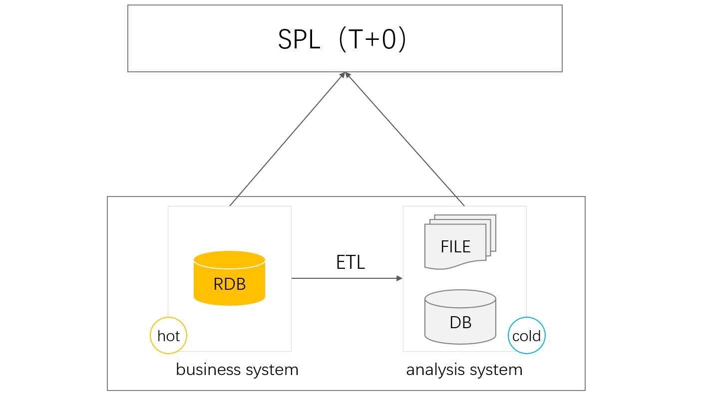
The single TP database naturally supports T+0 calculation. When there is too much data accumulation, it can affect the performance of the TP database. At this point, a portion of historical data is usually moved to a professional AP database, which is known as hot and cold data separation. The TP database only stores recently generated hot data, while the AP database stores historical cold data. After reducing the pressure on the TP database, it can run smoothly.
But in this way, when doing real-time whole-data statistics, cross database calculations are required, which has always been a hassle, especially when facing heterogeneous databases (TP and AP databases are usually not of the same structure). With esProc SPL’s mixed computing capability of different data sources, this problem can be easily solved.
| A | B | |
|---|---|---|
| 1 | =[[connect@l("oracle"),"ORACLE"],[connect@l("hive"),"HIVE"]] | |
| 2 | =SQL="select month(orderdate) ordermonth,sellerid,sum(amount) samount,count(amount) camount from sales group by month(orderdate),sellerid" | |
| 3 | fork A1 | =SQL.sqltranslate(A3(2)) |
| 4 | =A3(1).query(B3) | |
| 5 | =A3.conj().groups(ordermonth,sellerid;sum(samount):totalamount,sum(camount):totalcount) | |
For the mixed calculation between TP database Oracle and AP database Hive, SPL can also convert SQL into dialect syntax of different databases.
Then, how can the code written in esProc SPL be integrated into the application?
Very simple, esProc provides a standard JDBC driver, allowing Java programs to call SPL code just like calling database SQL.
Class.forName("com.esproc.jdbc.InternalDriver");
Connection conn =DriverManager.getConnection("jdbc:esproc:local://");
Statement statement = conn.createStatement();
ResultSet result = statement.executeQuery("=json(file(\"Orders.csv\")).select(Amount>1000 && like(Client,\"*s*\")
More complex SPL scripts can be saved as files, just like calling stored procedures:
Class.forName("com.esproc.jdbc.InternalDriver");
Connection conn =DriverManager.getConnection("jdbc:esproc:local://");
CallableStatement statement = conn.prepareCall("call queryOrders()");
statement.execute();
This is equivalent to providing a logical database without storage and without SQL.
SPL Official Website 👉 http://www.scudata.com
SPL Feedback and Help 👉 https://www.reddit.com/r/esProc
SPL Learning Material 👉 http://c.scudata.com
SPL Source Code and Package 👉 https://github.com/SPLWare/esProc
Discord 👉 https://discord.gg/ydhVnFH9
Youtube 👉 https://www.youtube.com/@esProc_SPL


Chinese version