The following Excel table has several columns of numbers:

Task: With a given parameter, find the first same number in each row and hide the columns on its right; if the number does not exist in a row, just hide the whole row. Below is the result when the given parameter is 100:

Use SPL XLL to enter the formula below:

=spl("=?1.(~.to(~.pselect(~==?2))).select(~!=[])",A1:C5,100)

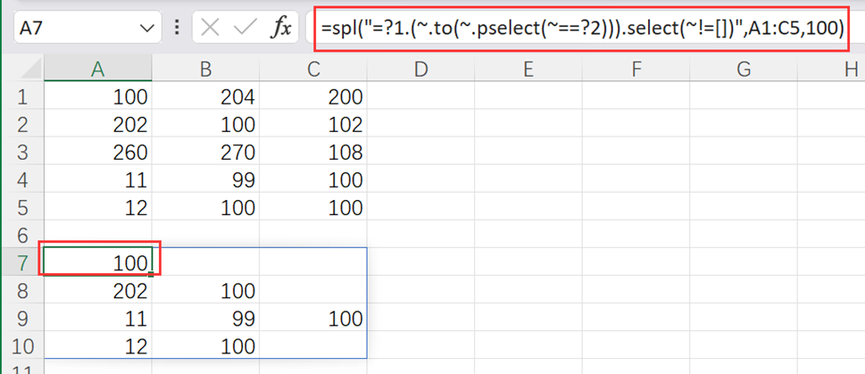
select()function gets members meeting the specified condition. pselect() function gets positions of the eligible members. to() function gets the first N members. ~ represents the current member.

The formula is used in scenarios where the table has unstandardized data, such as there are missing values in rows/columns and the rows/columns do not have fixed lengths. If there are more than one 100 in a row, columns on the right of the first 100 will be hidden by default. Use pselect@z if you need to hide columns on the right of the last 100.

Source:https://stackoverflow.com/questions/78274564/excel-formulas-how-to-grab-only-cells-to-the-left-of-a-value