Abstract

This series of articles explain how to perform multidimensional analysis (OLAP) in steps with detailed samples. Click to learn more in Multidimensional Analysis Backend Practice 1: Basic Wide Table. Multidimensional Analysis Backend Practice 1: Basic Wide Table

Aim of practice

 

This article aims at practicing how to build the basic wide table of the multidimensional analysis backend and access the wide table through SPL and SQL.

 

The steps of the practice are:

1. Prepare the basic wide table: retrieve the data of basic wide table from database and save them as a composite table file.

2. Access the basic wide table: access with SPL or SQL statements.

 

This article will take customer table as the sample wide table, and the SQL statement for retrieving wide table data from Oracle database is select * from customer. The execution result is as follows:

 

 

The fields include:

CUSTOMER_ID NUMBER(10,0), ID number of customer

FIRST_NAME VARCHAR2(20), first name

LAST_NAME VARCHAR2(25), last name

PHONE_NUMBER VARCHAR2(20), phone number

BEGIN_DATE DATE, date of beginning

JOB_ID VARCHAR2(10), job ID

JOB_TITLE VARCHAR2(32), job title

BALANCE NUMBER(8,2), balance

EMPLOYEE_ID NUMBER(4,0), ID number of employee

DEPARTMENT_ID NUMBER(4,0), ID number of department

DEPARTMENT_NAME VARCHAR2(32), name of department

FLAG1 CHAR(1), flag1

FLAG2 CHAR(1), flag2

FLAG3 CHAR(1), flag3

FLAG4 CHAR(1), flag4

FLAG5 CHAR(1), flag5

FLAG6 CHAR(1), flag6

FLAG7 CHAR(1), flag7

FLAG8 CHAR(1), flag8

mensional analysis calculation can be described in the following SQL statements of Oracle:

select department_id,job_id,to_char(begin_date,'yyyymm') begin_month ,sum(balance) sum,count(customer_id) count
from customer
where department_id in (10,20,50,60,70,80)
and job_id in ('AD_VP','FI_MGR','AC_MGR','SA_MAN','SA_REP')
and begin_date>=to_date('2002-01-01','yyyy-mm-dd')
and begin_date<=to_date('2020-12-31','yyyy-mm-dd')
and flag1='1' and flag8='1'
group by department_id,job_id,to_char(begin_date,'yyyymm')

Prepare wide table

Write etl.dfx to retrieve data from database and generate composite table file customer.ctx which is saved as the wide able. And the code is:

	A	B
1	=connect@l("oracle")	=A1.cursor("select   * from customer")
2	=file("data/customer.ctx").create@y(customer_id,first_name,last_name,phone_number,begin_date,job_id,job_title,balance,employee_id,department_id,department_name,flag1,flag2,flag3,flag4,flag5,flag6,flag7,flag8)
3	=A2.append(B1)	>A2.close(),A1.close()

 

A1: connect to the pre-configured oracle database. The @l option is used to process the field name to its lowercase, and please note l is the lower-case L rather than number 1.

B1: create a cursor based on the database, preparing to retrieve the data of customer table. customer is a fact table which is usually big in practice, so it needs to be retrieved with cursor to avoid memory overflowing.

A2: define a composite table file in columnar storage, and the field name is identical to B1.

A3: retrieve cursor B1 while exporting to composite table.

B3: close composite table and the database connection.

 

When there are one hundred million rows in the wide table, the exported composite table is about 3.5 GB.

 

Deploy esProc server

We first need to deploy esProc node according to the tutorials. Put meta.txt in main path and the file contents are the corresponding relations between the table name and the file name:

Table      File  Column  Type

customer       data/customer.ctx

The file name is relative to the main path. If the main path of node is d:/esproc/, then the entire file name will be d:/esproc/data/customer.ctx.

 

Access wide table

The multidimensional analysis backend needs to be invoked by a universal front-end. There are two methods of calling it: one is using SQL; the other is executing scripts, submitting parameters such as filter conditions, grouping fields, etc. to the backend for execution.

 

1. SQL

Let’s take a look at the first method and use the invoking of esProc JDBC in Java for example. The Java code sample is as follows:

public void testOlapServer(){
       Connection con = null;
       java.sql.Statement st;
       try{
              // create a connection
              Class.forName("com.esproc.jdbc.InternalDriver");
              // get the connection based on url
              con= DriverManager.getConnection("jdbc:esproc:local://?onlyServer=true&sqlfirst=plus");
              st = con.createStatement();
              // directly execute SQL+ statement to get the result set
              ResultSet rs = st.executeQuery("select department_id,job_id,year(begin_date)*100+month(begin_date) begin_month ,sum(balance) sum,count(customer_id) count from customer where department_id in (10,20,50,60,70,80) and job_id in ('AD_VP','FI_MGR','AC_MGR','SA_MAN','SA_REP') and (begin_date between timestamp('2002-01-01 00:00:00') and timestamp('2020-12-31 23:59:59')) and flag1='1'and flag8='1'group by department_id,job_id,year(begin_date)*100+month(begin_date)");
              // continue to process the result set to show it out
             
       }
       catch(Exception e){
              out.println(e);
       }
       finally{
              // close the connection
              if (con!=null) {
                     try {con.close();}
                     catch(Exception e) {out.println(e);       }
              }
       }
}

The customer.ctx here will be read in memory completely, which is not suitable for big data. /*+ external*/ can be added to the front of the table name for big data, and the composite table will be processed to a cursor. Or we can also execute the following script.

 

The SQL added with /*+ external*/ is as follows:

select department_id,job_id, string(begin_date,'yyyyMM'),sum(balance) sum,count(customer_id) count
from /*+ external*/ customer
where department_id in (10,20,50,60,70,80) and job_id in ('AD_VP','FI_MGR','AC_MGR','SA_MAN','SA_REP') and begin_date>=date('2002-01-01','yyyy-mm-dd') and begin_date<=date('2020-12-31','yyyy-mm-dd') and flag1='1' and flag8='1'
group by department_id,job_id, string(begin_date,'yyyyMM')

The total time of Java program execution is 88 seconds when using cursor.

 

It is worth noting that the absolute value of execution time here is not that important. We record the time just to calculate how much it can be reduced compared with the latter practice which uses multiple optimization methods.

 

We can execute SQL in multi-thread parallel by adding /*+parallel (n) */ to the table name. The complete two-thread parallel SQL is:

select department_id,job_id,year(begin_date)*100+month(begin_date) begin_month ,sum(balance) sum,count(customer_id) count
from /*+ external*/ /*+parallel (2) */ customer
where department_id in (10,20,50,60,70,80) and job_id in ('AD_VP','FI_MGR','AC_MGR','SA_MAN','SA_REP')
and (begin_date between timestamp('2002-01-01 00:00:00') and timestamp('2020-12-31 23:59:59'))
and flag1='1' and flag8='1'
group by department_id,job_id,year(begin_date)*100+month(begin_date)"

The execution time of Java program is 46 seconds in two-thread parallel.

 

2. Execute script

Multidimensional analysis front-end needs to call the entry script olap.dfx, and uses SPL to access the wide table and perform calculations of filtering, grouping and aggregating.

 

The front-end needs to pass customer, the name of the wide table, and other necessary information to olap.dfx though cellset parameters when calling the entry script. In the SPL code, the parameters given by front-end needs to be split to process and transform respectively for the purpose of better performance. Therefore, we use the json string, which is easy to split and parse, to pass other parameters expect for the separately given wide table name. It is also easy for the front-end to dynamically spell the parameters into json string.

 

Step one: write customer.dfx, and parse json string parameter.

Before writing olap.dfx, we need to write customer.dfx first to parse the given json string parameter. Since the parameters and processing methods of each wide table are not exactly the same, every wide table needs to correspond itself to a dfx file for parsing json string. And the dfx file name could be the same as the wide table name such as customer.dfx.

 

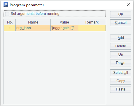
Define the cellset parameter arg_json, and put department ID number, job ID, flag bit, the range of date, grouping field and aggregate expression together in arg_json to pass them to SPL. The parameter setup window is as follows:

 

 The sample of arg_json parameter value is:

{
       aggregate:
              [
                     {
                            func:"sum",
                            field:"balance",
                            alias:"sum"
                     },
                     {
                            func:"count",
                            field:"customer_id",
                            alias:"count"
                     }
              ]，
       group:
              [
                     "department_id",
                     "job_id",
                     "begin_yearmonth"
              ],
       slice:
              [
                     {
                            dim:"department_id",
                            value:[10,20,50,60,70,80]
                     },
                     {
                            dim:"job_id",
                      value:["AD_VP","FI_MGR","AC_MGR","SA_MAN","SA_REP"]
                     },
                     {
                            dim:"begin_date",
                            interval:[date("2002-01-01"),date("2020-12-31")]
                     },
                     {
                            dim:"flag1",
                            value:"1"
                     },
                     {
                            dim:"flag8",
                            value:"1"
                     }
              ]
}

Description:

1. The name of composite table is passed as a separate parameter without putting it in json string.

2. “aggregate” is an array of aggregate expressions, and each member contains the field name “field”, aggregate function “func” and the alias “alias”.

3. “group” is an array of grouping fields. The data will be grouped by date if begin_date is a member or by year and month if begin_yearmonth is a member. They can be considered as two different fields for multidimensional analysis front-end.

4. “slice” is an array of slice expressions, and each member contains the dimension of slice “dim”, slice value (array or single value) or the range of “between” “interval”. Slice expressions are AND to each other.

 

The customer.dfx will return four strings, respectively “the field names used in the calculation”, aggregate expression, grouping expression and slice (filtering conditions) expression. Among them, the string “the field names used in the calculation” include all the fields used in aggregate expression and grouping expression without those used in slice expression. This string is used to define the fields retrieved from the cursor, and the fewer the fields are retrieved, the better the performance will be. The sample of SPL code is as:

	A	B		C
1	func
2		if A1.value==null	return "between("/A1.dim/","/A1.interval(1)/":"/A1.interval(2)/")"
3		else if ifa(A1.value)	return   string(A1.value)/".contain("/A1.dim/")"
4		else if   ifstring(A1.value)	return   A1.dim/"==\""/A1.value/"\""
5		else	return   A1.dim/"=="/A1.value
6	=json(arg_json)
7	=A6.aggregate.(~.func/"("/~.field/"):"/~.alias).concat@c()
8	=A6.group.(if(~=="begin_yearmonth","year(begin_date)*100+month(begin_date):begin_yearmonth",~)).concat@c()
9	=A6.aggregate.(field)	=A6.group.(if(~=="begin_yearmonth","begin_date",~))
10	=(A9|C9).id().concat@c()
11	=[]
12	for A6.slice	=[func(A1,A12)]	>A11|=B12
13	return A10,A7,A8,A11.concat("  &&")

Area from A1 to C5 is a subprogram which executes only when being called. We will explain them in the order of execution for the sake of better illustration.

 

A6: parse arg_json to table sequence. The result returned is a nested multi-layer table sequence as follows:

 

The “aggregate” in it is:

 

The “group” is:

 

And the “slice” is:

 

A7: first calculate “aggregate” to a sequence of colon-concatenated string as follows:

 

Then concatenate the sequence with commas to a string:

sum(balance):sum,count(customer_id):count

 

A8: replace begin_yearmonth in "group" with expression year(begin_date)*100+month(begin_date):begin_yearmonth. And concatenate the members of "group" to a string with commas: department_id,job_id, year(begin_date)*100+month(begin_date):begin_yearmonth.

 

A9: get the “field” in "aggregate", i.e. all the field names used in aggregate expression.

 

C9: replace begin_yearmonth in “group” with begin_date and the results are all the field names used in grouping expression.

 

A10: concatenate A9 and C9 together and continue to concatenate it with commas to a string in order to get all the required field names of the calculation: balance,begin_date,customer_id,department_id,job_id.

 

A11: define an empty sequence which prepares to store the sequence of slice (filtering conditions) expressions.

 

A12: loop through “slice” and the loop body is B12 and C12.

 

B12: use A12 (the current slice) as parameter to call subprogram A1.

 

B2: if the value of current slice is null, then it is between calculation. The return result of current C2 will be between(begin_date,date("2002-01-01"):date("2020-12-31")).

 

B3: if the value of current slice is sequence, then it is contain calculation. The return result of current C3 will be [10,20,50,60,70,80].contain(department_id) or ["AD_VP","FI_MGR","AC_MGR","SA_MAN","SA_REP"].contain(job_id).

 

B4: if the current slice is string, then it is string equivalence calculation. The return result of current C4 will be flag1=="1" or flag8=="1".

 

B5: if the current slice is none of the above, then it is numerical equivalence calculation. The current slice has no such a calculation, so we will illustrate another example: employee_id==2.

 

So far, the subprogram has done.

 

C12: append the result of A1 to A11. Continue the loop in A12 until it is over.

 

A13: return A11, A7, A8, and A11.concat("&&") respectively as:

 

The field names used in the calculation: balance,begin_date,customer_id,department_id,job_id

 

The aggregate expression: sum(balance):sum,count(customer_id):count

 

The grouping expression: department_id,job_id,string(begin_date,"yyyyMM"):begin_yearmonth

 

The slice expression: [10,20,50,60,70,80].contain(department_id) && ["AD_VP","FI_MGR","AC_MGR","SA_MAN","SA_REP"].contain(job_id) && between(begin_date,date("2002-01-01"):date("2020-12-31")) && flag1=="1" && flag8=="1"

 

Description: the calculations here include all the possibilities of OLAP slice with only slightly different writings of parameter. Other possibilities include:

 

1. The numeric “between” calculation such as the employee_id ranging from 100 to 200. Then the “slice” of arg_json needs to add:

            {
                      dim:"employee_id",
                      interval:[100,200]
               },

The result of func A1 will be: between(employee_id,100:200).

 

2. The date or numeric calculation of no less than or on more than such as  begin_date>= date("2002-01-01"). Then the “slice” of arg_json needs to add:

               {
                      dim:"begin_date",
                      interval:[date("2002-01-01"),]
               },

The result of func A1 will be: between(begin_date,date("2002-01-01"):).

 

Take employee_id<=200 for another example, and the “slice” of arg_json needs to add:

               {
                      dim:"employee_id",
                      interval:[,200]
               },

The result of func A1 will be: between(employee_id,: 200).

 

Step two: write olap.dfx to perform multidimensional analysis calculation.

 

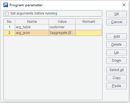
We first call customer.dfx in olap.dfx to parse json string and then operate OLAP calculation. The parameters of olap.dfx are arg_table and arg_json:

 

The SPL code is as follows:

 

	A
1	=call(arg_table/".dfx",arg_json)
2	=file("data/"/arg_table/".ctx").open()
3	=A2.cursor@m(${A1(1)};${A1(4)};2)
4	=A3.groups(${A1(3)};${A1(2)})
5	return A4

A1: call customer.dfx based on the value of arg_table parameter, and the parameter is arg_json. The return values are the above mentioned field name set and three expression strings.

 

A2: open the composite table object customer.ctx based on arg_table parameter.

 

A3: create a two-thread parallel cursor with the filter condition being a macro. The statement actually executed is:

=A2.cursor@m(balance,begin_date,customer_id,department_id,job_id;[10,20,50,60,70,80].contain(department_id) && ["AD_VP","FI_MGR","AC_MGR","SA_MAN","SA_REP"].contain(job_id) && between(begin_date,date("2002-01-01"):date("2020-12-31")) && flag1=="1" && flag8=="1";2)

 

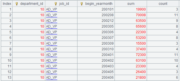
A4: operate small grouping and aggregation on A3. The statement actually executed is:

=A3.groups(department_id,job_id,string(begin_date,"yyyyMM"):begin_yearmonth }; sum(balance):sum,count(customer_id):count)

And the execution result is:

 

A5: return the result set of A4.

 

Step three: call from the front-end

After being written, olap.dfx needs to be called as a stored procedure during multidimensional analysis, and the Java code is as:

public void testOlapServer(){
       Connection con = null;
       java.sql.PreparedStatement st;
       try{
              // create a connection
              Class.forName("com.esproc.jdbc.InternalDriver");
              // get the connection based on url
              con= DriverManager.getConnection("jdbc:esproc:local://?onlyServer=true&sqlfirst=plus");
              // call the stored procedure, and olap is the file name of dfx
st =con.prepareCall("call olap(?,?)");
st.setObject(1, "customer");
st.setObject(2, "{aggregate: [{func:\"sum\",field:\"balance\",alias:\"sum\"},{func:\"count\",field:\"customer_id\",alias:\"count\"}],group:[\"department_id\",\"job_id\",\"begin_yearmonth\"],slice:[{dim:\"department_id\",value:[10,20,50,60,70,80]},{dim:\"job_id\",value:[\"AD_VP\",\"FI_MGR\",\"AC_MGR\",\"SA_MAN\",\"SA_REP\"]},{dim:\"begin_date\",interval:[date(\"2002-01-01\"),date(\"2020-12-31\")]},{dim:\"flag1\",value:\"1\"},{dim:\"flag8\",value:\"1\"}]}");//arg_json
// execute the stored procedure
st.execute();
// get the result set
ResultSet rs = st.getResultSet();
// continue to process the result set and show it out
             
       }
       catch(Exception e){
              out.println(e);
       }
       finally{
              // close the connection
              if (con!=null) {
                     try {con.close();}
                     catch(Exception e) {out.println(e);       }
              }
       }
}

Description: the multidimensional analysis front-end needs to concatenate a string beforehand to generate the value of arg_json parameter.

 

Here we are operating two-thread calculation, and we can also change olap.dfx to a single-thread calculation as follows:

A3 removes @m and the last parameter 2, but all else remains the same.

	A
1	=call(arg_table/".dfx",arg_json)
2	=file("data/"/arg_table/".ctx").open()
3	=A2.cursor(${A1(1)};${A1(4)})
4	=A3.groups(${A1(3)};${A1(2)})
5	return A4

For single-thread, the execution time of Java program plus background SPL is 84 seconds in total for 100 million data.

For two-thread, the execution time of Java program plus background SPL is 42 seconds in total.

 

Newly added data

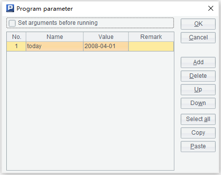
Every single day, the customer table have new data added which need to be added to the composite table file regularly. We can write etlAppend.dfx, and the cellset parameter is as:

 

The SPL code is as follows:

	A
1	=connect@l("oracle")
2	=A1.cursor("select   * from customer where begin_date=?",today)
3	=file("data/customer.ctx").open().append(A2)
4	>A3.close(),A1.close()

A1: connect to oracle database.

A2: create a cursor to retrieve the data of today.

A3: append today’s newly added data to the end of the composite table.

A4: close the file and database connection.

 

etlAppend.dfx needs to be regularly executed each day and the execution is done by using ETL tools or OS timed tasks to invoke esProc script from the command line.

 

For example:

C:\Program Files\raqsoft\esProc\bin>esprocx d:\olap\etlAppend.dfx