In the early days, some people used C++ or Java to develop quantitative trading strategy model. Currently, however, this field is almost monopolized by Python for the following two reasons:

Python provides convenient syntax and its operation interface is simple and easy to learn. After all, quantitative analysts are not yet professional programmer, and it is a bit too troublesome for them to master architecturally complex enterprise application development technology (Java/C++).

Python offers comprehensive libraries, such as Numpy and Pandas for data analysis and processing, Matplotlib and Seaborn for visualization, TA-Lib for financial technical analysis, scikit-learn for machine learning, and TensorFlow and Pytorch for deep learning. These libraries, especially the data algorithm related libraries, provide strong support for the implementation of quantitative trading strategies.

However, Python is not perfect, as reflected in the following aspects.

Some Python codes are still quite complex. For example, Python is deficient in loop functions, so it often needs to use the for loop to hard-code; since neither Python itself nor third-party libraries provide methods to solve some common operations like adjacent reference, positioning calculation, and ordered grouping, it has to hard-code or select a roundabout solution when encountering such operations.

Debugging in Python is not very convenient. While Python offers many IDEs, and all of them have the debugging function, ‘print method’ is still the most frequently employed method, which is always very cumbersome.

Python is also deficient in big data methods. When the amount of data is too large to fit in the memory of one machine, it has to hard code and process in segments, resulting in difficulty to code and unsatisfactory running efficiency. Moreover, Python doesn’t have true parallel computing ability, and its multi-thread computing is actually still single-thread computing. If we want to implement true parallel computing, we can only use multiple processes, which is an almost impossible task for quantitative analysts.

So, besides Python, are there any other programming languages that can be used for quantitative trading strategy?

Yes, esProcSPL, which can overcome these shortcomings of Python.

esProcSPL is a programming language specifically for the computation of structured data, which has the following advantages: i)it boasts more convenient syntax than Python, allowing beginners to code within just two or three days, and truly achieving simple coding; ii) it offers complete operations, especially those order-based operations, all of which are elaborately designed, including adjacent reference, ordered grouping, and positioning calculation, etc.; iii)it provides consistent syntax, making it easy to code; iv) it is a grid-style programming language, allowing for real-time review of the result in each cell without the need to use ‘print’, and making code debugging convenient and fast; and v) it provides very comprehensive support for big data and parallel computing. The only fly in the ointment is that SPL currently lacks sufficient support for machine learning algorithm.

More agile code

SPL’s agile syntax is reflected in all aspects of code writing, such as set operations and lambda syntax. Instead of presenting a comprehensive introduction here, we only take the lambda syntax as an example to illustrate.

Let’s look at some common calculations in quantitative analysis.

Example 1: Assume the following sequence is the stock price of a certain stock for one month. Now we want to calculate the daily rise and fall of the stock price for this month. Here it is stipulated that the rise on the first day is 0.

Look at the Python code first:

close=[12.99,12.72,12.7883,12.5931,13.2081,13.1105,12.8371,13.0421,13.3741,12.7981,12.925,12.9152,12.7883,13.0226,12.7298,12.4564,12.5833,12.6419,12.6712,12.4662,12.7981,12.8274]
s = pd.Series(close)
ss = s.shift()
ma = (s-ss).fillna(0).max()

SPL code:

	A
1	[12.99,12.72,12.7883,12.5931,13.2081,13.1105,12.8371,13.0421,13.3741,12.7981,12.925,12.9152,12.7883,13.0226,12.7298,12.4564,12.5833,12.6419,12.6712,12.4662,12.7981,12.8274]
2	=A1.(if(#==1,0,~-~[-1])).max()

SPL uses # to represent the sequence number of current member, ~ to represent current member, and [] to obtain adjacent member. This code is very concise. In contrast, Python’s Lambda syntax cannot obtain the said three values at the same time, so it can only shift the index first, and then fill the null with 0, which makes the code writing slightly cumbersome.

Example 2: Calculate the rise of a stock in three days when its prices is maximum.

Python code:

stock_prices = [12.99, 12.72, 12.7883, 12.5931, 13.2081, 13.1105, 12.8371, 13.0421, 13.3741, 12.7981, 12.925, 12.9152, 12.7883, 13.0226, 12.7298, 12.4564, 12.5833, 12.6419, 12.6712, 12.4662, 12.7981, 12.8274]
top_three_days = sorted(range(len(stock_prices)), key=lambda i: stock_prices[i],reverse=True)[:3]
increases = [stock_prices[i] / stock_prices[i-1] -1 if i!=0 else None  for i in top_three_days]

SPL code:

	A
1	[12.99,12.72,12.7883,12.5931,13.2081,13.1105,12.8371,13.0421,13.3741,12.7981,12.925,12.9152,12.7883,13.0226,12.7298,12.4564,12.5833,12.6419,12.6712,12.4662,12.7981,12.8274]
2	=A1.ptop(-3,~)
3	=A1.calc(A2,if(#==1,null,~/~[-1]-1))

Python needs to sort by stock price first to find the indexes of the top three stock prices, and then write a for loop to calculate the rise rate.

SPL first uses ptop()to directly find the indexes of the three days with the highest stock price without big sorting action involved, and then locates the said three indexes directly with the calc function, and finally employs [] to get adjacent members to calculate the rise rate. This code is simple to write and clear.

Example 3: Calculate the maximum number of days that a stock keeps rising:

Python code:

stock_prices = [12.99, 12.72, 12.7883, 12.5931, 13.2081, 13.1105, 12.8371, 13.0421, 13.3741, 12.7981, 12.925, 12.9152, 12.7883, 13.0226, 12.7298, 12.4564, 12.5833, 12.6419, 12.6712, 12.4662, 12.7981, 12.8274]
max_days = 0
current_days = 1
for i in range(1, len(stock_prices)):
if stock_prices[i] > stock_prices[i - 1]:
        current_days += 1
else:
        max_days = max(max_days, current_days)
        current_days = 1
max_days = max(max_days, current_days)

SPL code:

	A
1	[12.99,12.72,12.7883,12.5931,13.2081,13.1105,12.8371,13.0421,13.3741,12.7981,12.925,12.9152,12.7883,13.0226,12.7298,12.4564,12.5833,12.6419,12.6712,12.4662,12.7981,12.8274]
2	=A1.group@i(~<~[-1]).max(~.len())

Because Python lacks basic method to solve order-related operations, it has to hard-code. SPL, by contrast, provides the group@i()method, which will re-group once the condition changes (stock price falls). Therefore, the in-group number of members is the number of days that the stock price rises. Comparing the two codes, it’s clear which one is more agile.

Easier installation, more convenient debugging

Let’s start with installation. It’s still a bit difficult to install Python. Installing the basic parts of Python is relatively simple – just follow the instructions on the Internet to install step by step, and it is not a problem for most people except it may take a while. However, the installation of third-party libraries is not very simple. Due to the lack of unified management of Python versions and third-party library versions, it is common to encounter compatibility issues between Python version and library version, or between library versions. If encountering such issue, the issue alone will be challenging to resolve.

The installation of SPL is almost foolproof. After downloading the installation package from official website, you just need to click ‘Next’ all the way to complete the installation.

Now let’s talk about debugging. Python provides many IDEs, the most commonly used ones include Pycharm, Eclipse, Jupyter Notebook, etc. Each IDE has its own advantages and disadvantages, but the most commonly used debugging method of Python is still ‘print’ (print the variable values we want to watch), which is troublesome, and the print code needs to be deleted after debugging. The setting and execution of breakpoint are the normal functionality of Python IDEs, which is useful for debugging. It is worth noting that most IDEs of Python provide the functionality of completing variables and functions, which can save a lot of time when coding.

The following figure is the IDE of Pycharm:

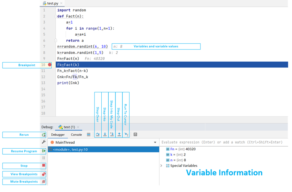
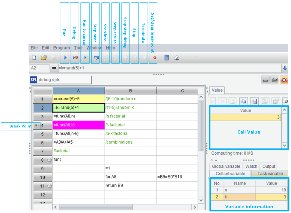
SPL adopts the grid-style programming, allowing us to view cell value and variable value at any time, and to code while looking at the results of the previous step. This method is much more convenient than the print method. As for the setting and execution of breakpoint, SPL’s IDE differs little from Python’s IDE. What needs to be improved is the completing functionality of function name and variable name.

Here below is the IDE of SPL:

More complete big data and parallel computing capabilities

Python lacks support for big data computing, and its parallel computing is fake. SPL, by contrast, has a complete cursor mechanism, which can process big data easily. Moreover, most of the cursor functions are used almost the same way as memory functions and very user friendly.

Let’s take an example: View the total net assets of each industry.

SPL code:

	A
1	=file("all_stock_info.csv").cursor@tc()
2	=A1.groups(industry;sum(total_assets):assets)

From the code in A2 alone, we cannot distinguish it is an in-memory calculation or a cursor calculation, because this code is the exactly the same as that used in in-memory calculation. SPL encapsulates operations on big data into a form that is essentially the same as in-memory operation, reducing the complexity of users to memorize.

Writing the parallel computing code in SPL is also very simple. For example, to perform the above calculation in parallel, just add the @m option to A1 (cursor@tcm()) and leave the code of A2 unchanged.

SPL’s shortcomings and supplementary tool ‘YModel’

Compared with Python, the machine learning ability of SPL is weak. Although SPL supports some common machine learning algorithms, such as supervised learning algorithms (linear regression, ridge regression and support vector machine), and unsupervised learning algorithms (k-means clustering, etc.), it doesn’t support some complex models like GBDT and XGB. This may pose some challenges in the implementation of quantitative trading strategies.

However, as far as quantitative analysis is concerned, particularly complex machine learning algorithms and even deep learning are usually only used by a few large institutions. For most quantitative analysts, trading strategies are not that complicated, and general strategies can all be implemented using SPL. If a particularly complex machine learning model is indeed required, SPL can call the interface of YModel to build a complex model and accomplish prediction.

YModel is an automatic modeling software, which can automatically carry out preprocessing and model building with just one click. With YModel, there is no need to worry about missing value, outlier, high cardinality variable, time feature, algorithm selection, parameter optimization, etc., because YModel will automatically process all of them. YModel offers common machine learning and deep learning models, and the models it builds can rival those created by professional algorithm engineers, which greatly reduces the cost of learning algorithm and helps financial traders who are proficient in trading strategies but unfamiliar with algorithms save a lot of time so that they can focus more on researching trading strategies instead of complex mathematical algorithms. By calling the automatic modeling interface of YModel, SPL and YModel work together to implement the development and testing of trading strategy conveniently and efficiently.

Take a simple example of using SPL and YModel to build a model to perform a machine learning trading strategy:

Predict the market value of a company based on five indexes: working capital, net debt, price-to-book ratio, net return on total assets, and turnover rate. If the predicted market value is much higher than the actual market value, the market value is considered undervalued; otherwise, the market value is considered overvalued.

Assume we have organized these data using SPL, the feature variables are net asset, debt to asset ratio, net profit, net profit rate and profit growth rate, and the target variable is the company’s market value.

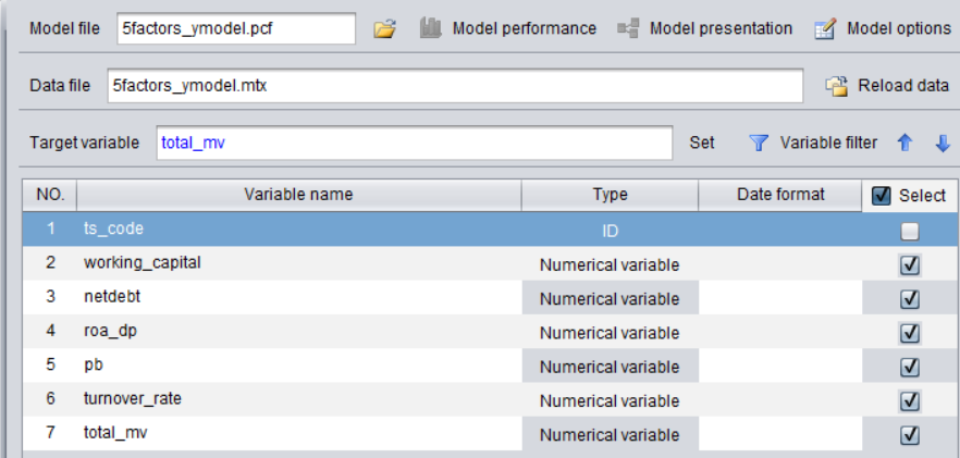
Configure YModel modeling parameters and uncheck the stock code (ts_code):

Select a model (In most cases, the default settings are sufficient).

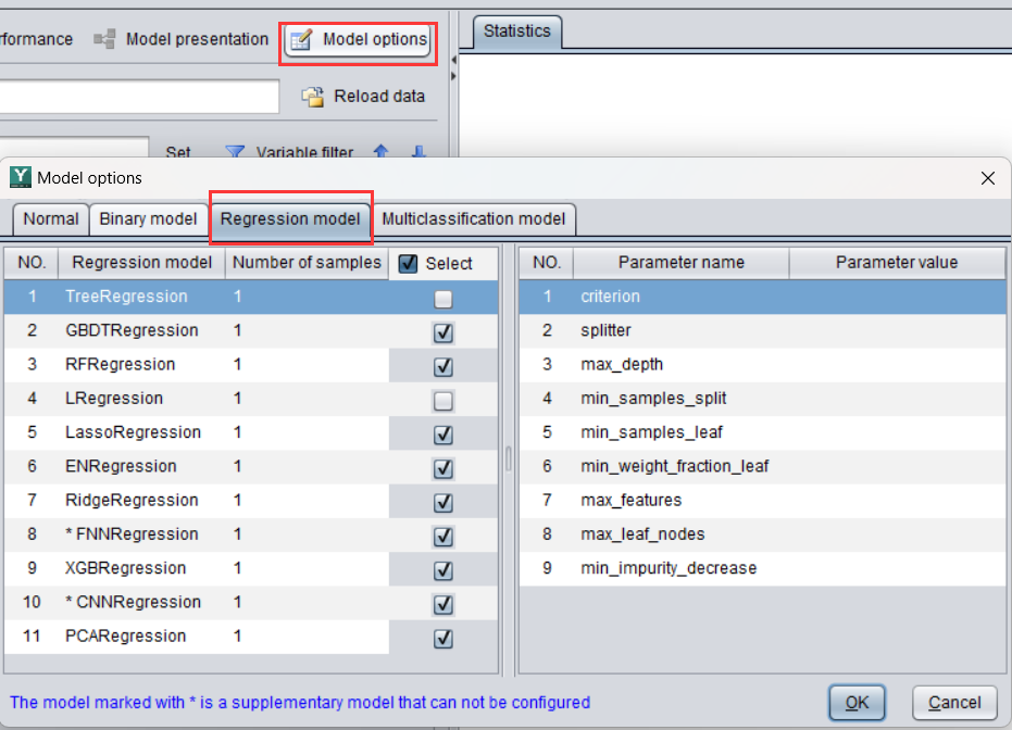
Use the information to generate an information model parameter file (.mcf).

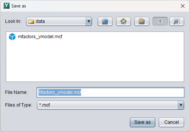
Model and predict in SPL:

	A
1	=ym2_env("D:/Ymodel/ymodel")
2	=ym2_mcfload("D:/Ymodel/ymodel/data/5factors_ymodel.mcf")
3	=ym2_model(A2)
4	=ym2_pcfsave(A3,"D:/Ymodel/ymodel/data/5factors_ymodel.pcf")
5	=ym2_pcfload("D:/Ymodel/ymodel/data/5factors_ymodel.pcf")
6	=ym2_predict(A5,"D:/Ymodel/ymodel/data/5factors_ymodel.csv")
7	=ym2_result(A6)
8	>ym2_close()
9	=A7.derive(1-total_mv_predictvalue/total_mv:diff_rate)
10	=A9.sort(diff_rate)

A1: Initialize the environment.

A2: Load model parameter (mcf file).

A3: Automatic modeling.

A4: Save the model file (pcf file).

A5: Load the model file.

A6: Use the model to make prediction on the new data in the csv file.

A7: Predicted result.

The red box in the figure is the target variable (market value); the blue box is the result predicted by YModel (predicted market value).

SPL first gets the data file ready, and then YModel performs the above modeling and prediction operations, and finally SPL analyzes the predicted result. The whole process runs smoothly and efficiently. Using SPL and YModel to perform quantitative analysis is much faster than using Python to independently perform data processing (missing value, outlier, high cardinality, etc.), model selection, and parameter adjustment. For ordinary quantitative analysts, the model built by YModel is accurate enough.