

DQL Practices: Metadata and Syntax
Ⅰ Prepare data
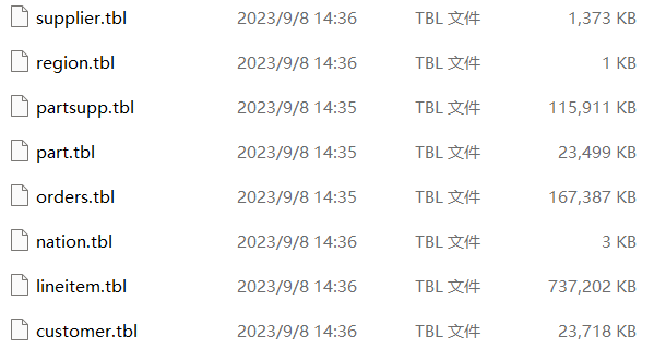
We use 1GB TPC-H data to show how to make DQL queries. Below are eight data files (*.tbl) generated by TPC-H:
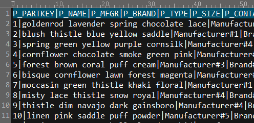
The file content is of text format. The first row contains field names and rows after it are detail data; and each row of data is separated by the vertical bar |. As shown in the following part table:
The data table queried in DQL should be stored in SPL composite table file format (*.ctx). We can use the following SPL script to convert text files to a composite table file:
| A | B | C | |
| 1 | E:\TPCH\ | ||
| 2 | 1024 | supplier | #S_SUPPKEY,S_NAME,S_ADDRESS,S_NATIONKEY,S_PHONE,S_ACCTBAL,S_COMMENT |
| 3 | 1048576 | partsupp | #PS_PARTKEY,#PS_SUPPKEY,PS_AVAILQTY,PS_SUPPLYCOST,PS_COMMENT |
| 4 | 1048576 | part | #P_PARTKEY,P_NAME,P_MFGR,P_BRAND,P_TYPE,P_SIZE,P_CONTAINER,P_RETAILPRICE,P_COMMENT |
| 5 | 1048576 | orders | #O_ORDERKEY,O_CUSTKEY,O_ORDERSTATUS,O_TOTALPRICE,O_ORDERDATE,O_ORDERPRIORITY,O_CLERK,O_SHIPPRIORITY,O_COMMENT |
| 6 | 1048576 | lineitem | #L_ORDERKEY,#L_LINENUMBER,L_PARTKEY,L_SUPPKEY,L_QUANTITY,L_EXTENDEDPRICE,L_DISCOUNT,L_TAX,L_RETURNFLAG,L_LINESTATUS,L_SHIPDATE,L_COMMITDATE,L_RECEIPTDATE,L_SHIPINSTRUCT,L_SHIPMODE,L_COMMENT |
| 7 | 1048576 | customer | #C_CUSTKEY,C_NAME,C_ADDRESS,C_NATIONKEY,C_PHONE,C_ACCTBAL,C_MKTSEGMENT,C_COMMENT |
| 8 | 1024 | nation | #N_NATIONKEY,N_NAME,N_REGIONKEY,N_COMMENT |
| 9 | 1024 | region | #R_REGIONKEY,R_NAME,R_COMMENT |
| 10 | =create(size,tblName,fields).record([A2:C9]) | ||
| 11 | for A10 | =file(A1/A11.tblName/".tbl").import@t(;,"|") | |
| 12 | =file(A1/A11.tblName/".ctx").create(${A11.fields};;A11.size) | ||
| 13 | >B12.append(B11.cursor()),B12.close() | ||
Lines 2~9 define 8 tables. Column A defines composite table block sizes; set block size corresponding to a table having a very small amount of data as 1KB and block sizes corresponding to the other tables as 1MB. Column B contains table names. Column C has field names, where one beginning with # is a primary key dimension field.
Write data of the 8 tables to A10’s table sequence.
Lines 11~13 import those tables one by one, create a composite table and write text data to the composite table file.
Ⅱ Create DQL metadata file
Create pseudo tables
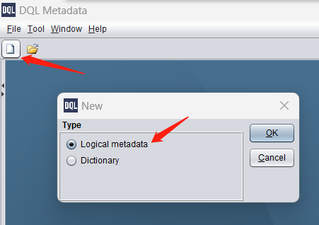
Open the DQL designer and create a new metadata file:
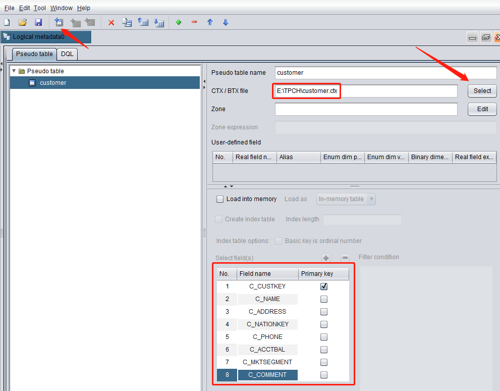
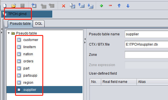
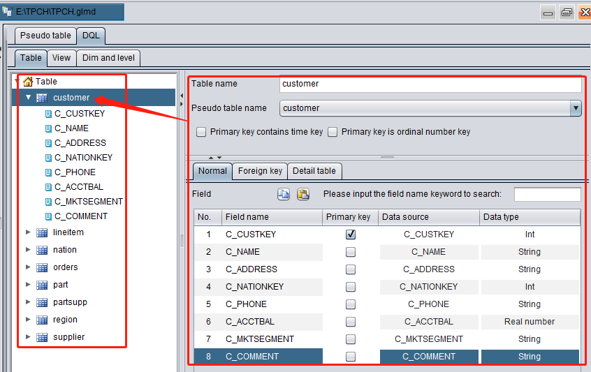
Select the newly-generated customer.ctx file and add a pseudo table. Its fields and primary key will be automatically identified:
Load the other tables in the same way. Save the metadata file as TPCH.glmd:
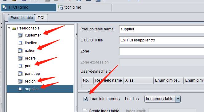
Select “Load into memory” for each of customer, nation, part, region and supplier tables. DQL requires that dimension tables be loaded into the memory in advance (pseudo tables do not have such a requirement):
Configure DQL tables
Import pseudo tables
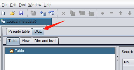
Switch to DQL tab, where there are no tables:
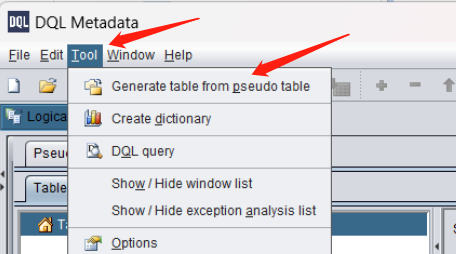
On the menu, click “Tool -> Generate table from pseudo table”:
Select all pseudo tables just loaded:
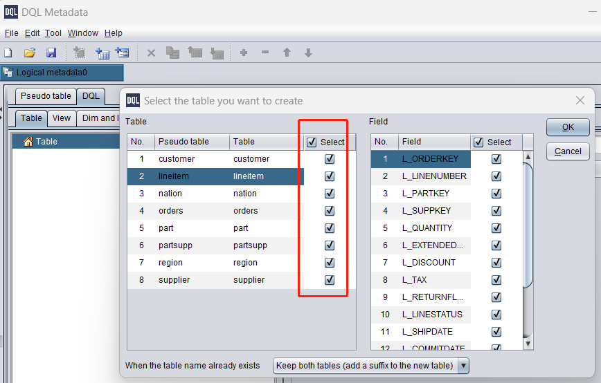
DQL tables are successfully created. And their primary keys and field data types are automatically identified:
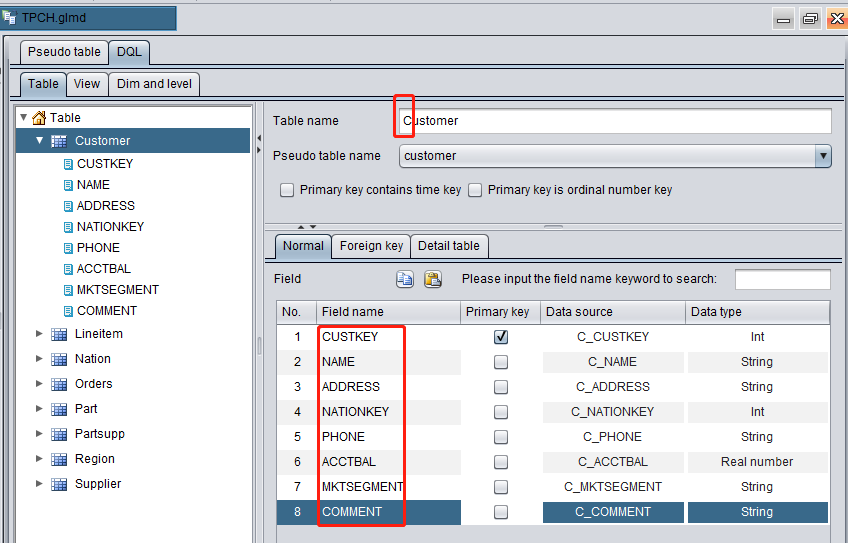
Adjust table names and field names slightly by changing the first letter of each table name to Capital and removing the suffix, such as “C_”, from each field name:
Create logical dimension tables: Year, Month and Day
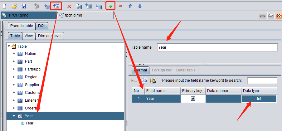
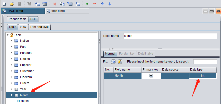
It is common to group data by year, month or day during a query. Therefore, we need to define these dimensions beforehand. On the toolbar click “Add” button to add a logical table. Set table name as Year, add a field also named Year and set as the primary key, and select Int as the field data type:
Add dimension table Month in the same way. The Month dimension contains year information and is also integer type. 202308, for example, represents August 2023:
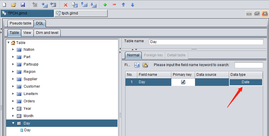
Mostly the date field in the other tables is of date type, so just set it as date type instead of the integer type like 20230815:
Set inter-table relationship
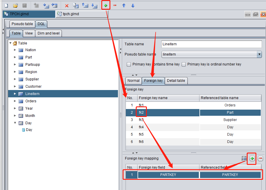
Select Lineitem table, switch to “Foreign key” tab to add the foreign key and set association relationship for each foreign key. Foreign key fk1, for example, is the relationship between Lineitem’s PARTKEY field and dimension table Part’s primary key PARTKEY field:
After the foreign key mapping is set up for all tables, switch to “View” tab where all grouping dimensions are listed in the middle and DQL tables are listed on both sides. Each DQL table matches to all grouping dimensions it involves through lines:
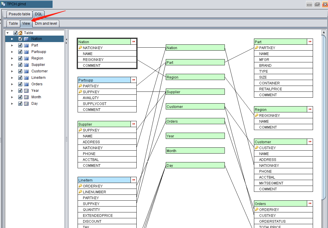
Both an ordinary ER diagram and this diagram show association relationships for each table. But DQL introduces the concept of grouping dimension to draw the above bus relationship diagram.
Supplier table and Customer table associate with Nation table through their foreign keys. *Nation *table is a dimension table and Nation is a grouping dimension. The NATIONKEY field in each of the three tables stores values of the Nation dimension.
Dimension tables will be randomly accessed during computations. DQL (the low-level SPL) requires to load dimension tables to the memory in advance. Generally, the size of dimension tables is relatively small and can fit into the memory.
Configure dimensions and dimension levels
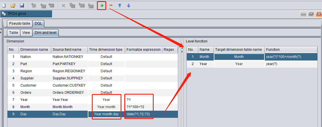
Switch to “Dim and level” tab where three time dimensions – Year, Month and Day – should be configured:
The time dimension type of Year dimension is Year. The formatted expression ?1 represents the year;
The time dimension type of Month dimension is Year month. Using the formatted expression ?1 (Year) *100 + ?2 (Month), we will have a Year month value like 202308;
The time dimension type of Day dimension is Year month day. Use SPL function date(year,month,day) to compute the date type Year month day value;
We can use the level function to compute the Month dimension and Year dimension according to the Day dimension. In the level function year(?)*100+month(?) for computing the Month dimension, question mark ? represents the current Year month day value. In SPL, month(date) function gets the Year month value from the specified data and year(date) function gets the Year value from the specified date.
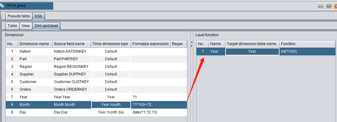
Likewise, we can use the level function int(?/100) to compute the Year dimension according to the Month dimension:
Save TPCH.glmd, and based on this metadata file we can perform DQL queries. Deploy the file on DQL server and the application can provide the external query service via JDBC.
Ⅲ Test DQL queries
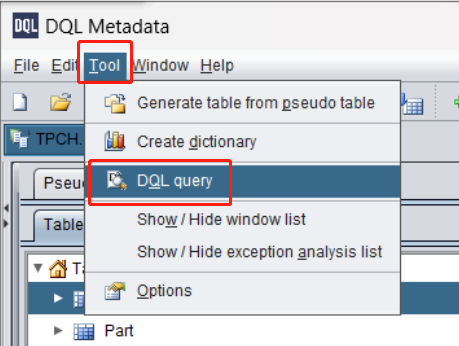
After the DQL metadata file is created, we can test the DQL query through “Tool –> DQL query”:
DQL query example 1
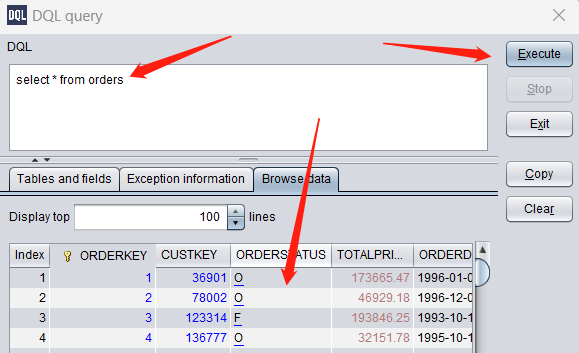
Write a simple DQL query manually, click “Execute” and result is displayed below:
DQL query example 2 – Generalized field
Let’s look at a more complicated query. orderkey is the primary key field of Orders table;
Use level function year to get Year dimension, which is the order year orderdate#year, according to Day dimension field orderdate;
Query customer name custkey.name through foreign key field custkey. The generalized field custkey.name will automatically associate Customer table during the actual query;
The generalized field query can have more than one level, such as custkey.nationkey.regionkey.name, which finds name of the region where order customer’s nation is located. The four involved tables – Orders, Customer, Nation and Region – will be automatically associated:
SELECT
   orderkey,
   orderdate#year orderyear,
   custkey.name custname,
   custkey.nationkey.regionkey.name regionname
FROM Orders
DQL example 3 – Grouping & Aggregation by dimension/dimension level
Compute the minimum discount and the total quantity according to month dimension and supplier dimension. The BY subclause specifies month in shipdate and suppkey as grouping fields:
SELECT
   MIN(discount) ,
   SUM(quantity)
ON
   month,
   supplier
FROM Lineitem
   BY shipdate#month, suppkey
The month dimension value is computed from the day dimension shipdate using level function month. The level function month can be omitted and DQL will automatically find the appropriate level function to perform the computation. Therefore, the BY subclause can be simply written as BY shipdate, suppkey.
DQL example 4 – Alignment aggregation on two (multiple) tables by same dimension
Supplier table and Customer table do not have direct association. But it is still possible to perform grouping & aggregation on them according to the same dimension. To count suppliers and customers according to nation:
SELECT
   COUNT(s.name) suppNum,
   COUNT(c.name) custNum
ON
   nation
FROM
   Supplier s BY nationkey
   UNION
   Customer c BY nationkey
DQL example 5 – Specify conditions on detail data/Perform filtering & aggregation/Sort result set/Get the first N records
Based on example 5, we add some commonly used query functionalities:
Specify conditions on detail data: WHERE nation>5;
Perform grouping & aggregation: HAVING suppNum>400;
Sort result set: ORDER BY custNum desc;
Get the first N records: LIMIT 10;
SELECT
   COUNT(s.name) suppNum,
   COUNT(c.name) custNum
ON
   nation WHERE nation>5
FROM
   Supplier s BY nationkey
   UNION
   Customer c BY nationkey
HAVING suppNum>400
ORDER BY custNum DESC
LIMIT 10
Summary
Create DQL metadata file correctly, deploy it on DQL server and provide external query service via JDBC. The DQL query service is generally needed by some WEB business systems.
In the next essay, we will illustrate how to apply DQL query service in WEB systems and, furthermore, visualize the DQL query model on the WEB page, where the WEB user selects information needed to automatically generate a DQL statement and query the target data from the DQL server.
The DQL query model conforms more to the natural way of thinking people use to deal with the real-life businesses, which makes the DQL visual query tool easier and more flexible to use.
SPL Official Website 👉 https://www.scudata.com
SPL Feedback and Help 👉 https://www.reddit.com/r/esProcSPL
SPL Learning Material 👉 https://c.scudata.com
SPL Source Code and Package 👉 https://github.com/SPLWare/esProc
Discord 👉 https://discord.gg/2bkGwqTj
Youtube 👉 https://www.youtube.com/@esProc_SPL


Chinese version