The objective of this practice is to search for the member with the highest similarity to the target vector from a large number of high-dimensional (such as 512-dimensional) binary vectors. A binary vector refers to the vector whose dimension values are either 0 or 1; the similarity refers to being close in distance in high-dimensional space. There are many types of distances, such as Euclidean distance, Mahalanobis distance and cos similarity, among which, the cos similarity is the most commonly used method in the industry to measure the similarity between vectors. The larger the cos similarity, the closer the distance and the more similar the two vectors are.

Due to the inability to define a distance-related order on high-dimensional vector dataset, it is impossible to build an efficient index as relational database does. In this case, the only way to find the nearest member is to traverse all data, yet it will result in poor performance when the amount of data is large.

In order to solve this problem, the professional vector database is usually adopted in the industry. The vector database has some built-in ANN (Approximate Nearest Neighbor) algorithms used for searching for vector, making it very possible to quickly find the member nearest to the target vector. Though it cannot guarantee a 100% chance of finding the desired member, this approximate solution is already sufficient for most application scenarios.

However, the vector database is very complex and heavy, and the number of ANN algorithms is large (different similarity problems require different ANN algorithms) and, the algorithm itself has many parameters, so in practice, it is almost impossible to select the right ANN algorithm and adjust its parameters in one attempt. Instead, we need to test repeatedly. Once the selected ANN algorithm fails to meet the requirements, we need to redefine the distance and choose another algorithm or resort to other solutions, all of which exceed the scope of vector database.

SPL has flexible and efficient computing ability and provides a wealth of computing functions, making it possible to handle such problems conveniently. Instead of researching, deploying, installing, and debugging vector database, it is better to adopt SPL.

Store data as bits

The binary vector can be stored as bits, with each dimension occupying only one binary bit. In this way, the storage amount can be reduced, and utilizing bitwise operation can yield a substantial improvement in computing efficiency.

A 512-dimensional binary vector takes up 512 binary bits, i.e., 64 bytes. In SPL, it can be represented by a long sequence of length 8.

The following code is to convert a batch of 512-dimensional binary vectors to long sequence, and store in SPL’s btx file.

	A
1	=directory@p("raw_data")
2	=A1.(file(~).read@b())
3	=A2.(blob(~))
4	=A3.new(filename@n(A1(#)):name,~.bits():data)
5	=file("longdata.btx").export@b(A4)

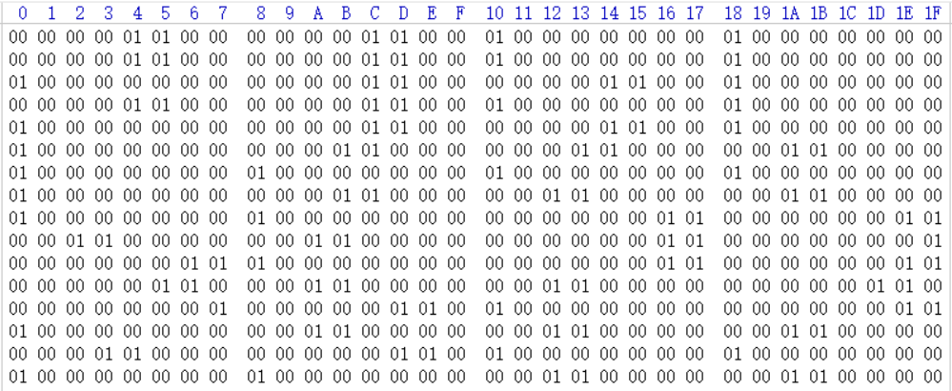
The raw_data refers to the storage directory of raw data, in which each file corresponds to one vector; the file name is the identity of vector; the file length is 512 bytes; each byte corresponds to one dimension. The form is as follows:

A1: list the file names under the directory

A2: read files

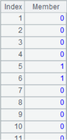
A3: convert each piece of data to a binary sequence of length 512 in the following form:

A4: create a table sequence, in which the name field is the identity of vectors, i.e., the file name; the data field is the sequence consisting of 8 long integers converted from 512-dimensional binary sequence. The form of table sequence is as follows:

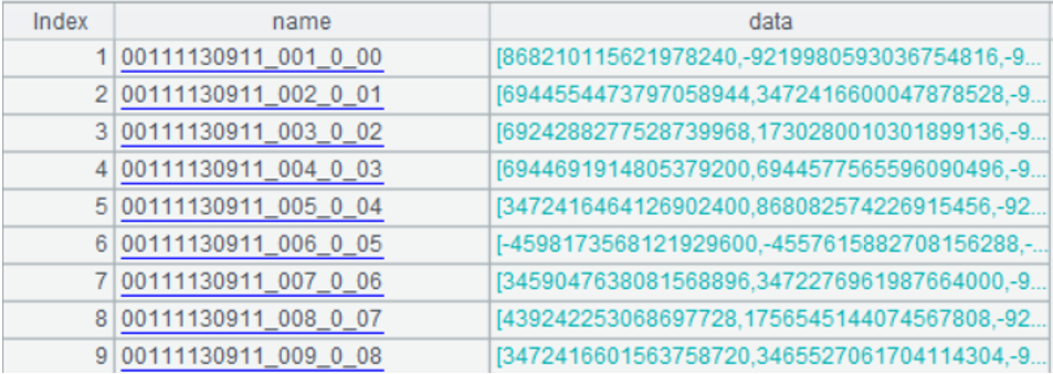
Here below is the sequence at the first row of data field:

The amount of data to be tested is around 900,000 rows, and the converted longdata.btx is a binary file containing 900,000 rows and 2 columns, about 11M in size.

Convert the target vectors for testing in the same way and generate the “target_vec.btx” file to facilitate subsequent comparison.

Replace cos similarity with XOR distance

This industry usually uses the cos similarity to measure the similarity between two vectors. However, since the topic we are discussing is somewhat special, that is, the dimension values in a vector are either 0 or 1, the cos similarity results can deviate significantly from our intuitive feelings. For example, when the number of dimension value 1 is large, and only a few dimensions are different, the calculated cos similarity will be very large; on the contrary, when the number of dimension value 0 is large, and only a few dimensions are different, the calculated cos similarity will be much smaller.

Let’s take two sets of 8-dimensional vectors as an example:

x1=11111100
x2=11111010

x1 and x2 are different in only two dimensions, and their cos similarity is 0.833.

x3=00000011
x4=00000101

Likewise, x3 and x4 are different in only two dimensions, but their cos similarity is only 0.5.

We can see that both sets of vectors differ in only two dimensions, giving us an intuitive feeling that their cos similarity results should be the same but, the calculation results are quite different in fact. When the number of dimensions is larger, the gap will widen.

In order to make the result conform more to intuitive feeling, we adopt the XOR distance to measure the similarity between vectors. XOR distance refers to the number of dimensions whose value is different from the one at the corresponding bit between two vectors. For example, both the XOR distances between x1 and x2, and x3 and x4 are 2 in the above example, indicating the similarities of the two sets of vectors are the same.

SPL provides the bit1() function, which can conveniently calculate the XOR distance between two sequences. In the following text, any distance refers to the XOR distance unless otherwise specified.

Calculate XOR distance in SPL:

	A
1	=512.(rand(2))	/Binary vector 1
2	=512.(rand(2))	/Binary vector 2
3	=A1.bits()	/long data sequence 1
4	=A2.bits()	/long data sequence 2
5	=bit1(A3,A4)	/XOR distance

Another benefit of XOR distance is that it involves only bit operation and does not involve division operation compared to cos similarity, so the result can be figured out more quickly.

An attempt to cluster

The ANN algorithms are usually divided into two parts:

1. Clustering: divide data into different subsets according to certain rules so as to make the points in such a subset closer and make the points in two subsets farther apart. In layman’s terms, it is to put the data that are close to each other in a group and make the distance between the groups as far as possible.

2. Query: when querying the vector that is most similar to the target vector, it only needs to traverse the subsets nearest to the target vector, without having to traverse all the data. Although doing so may sometimes fail to find the nearest member, there is a high probability, which is the trade-off between efficiency and accuracy.

K-means is the most commonly used clustering method, which requires the number of clusters (k) to be determined in advance. However, pre-determining k value is difficult for the task we are discussing, as it requires a large number of attempts to find the correct k value. In addition, it also needs to calculate the center of mass during the k-means clustering process, yet the center of mass of binary vector is not easy to define. Taken together, we believe that k-means algorithm is not well-suited for the current problem.

Therefore, we decide to develop our own clustering method; the approximate process is as follows:

We will try to split data into N subsets, and the threshold for the number of members in each subset is M.

1. Denote all data as the set X, and randomly select one vector as the first base vector _x_1. Now the current set X can also be called the first subset _X_1.

2. From _X_1, find the vector farthest from the base vector and let it be the base vector _x_2 of the 2nd subset _X_2.

3. When there are i subsets, calculate the distance between every vector and each base vector xi, and put the vector nearest to a certain base vector into the subset that this base vector belongs to.

4. The base vector xi+1 of the (i+1)th subset _X_i+1 is obtained in a way that first finds the subset with more than M members and largest radius from the existing i subsets, and then selects the vector farthest from its base vector from the found subset as the base vector xi+1 of the (i+1)th subset (the radius of a subset is defined as the maximum of all distances between every member of the subset to its base vector).

5. Repeat steps 3 and 4 until the number of members of every subset is less than M or the number of subsets reaches N.

When calculating distances (the nearest distance in step 3 and the farthest distance in step 4), there may be a situation where the distances are equal. In this case, add a random number to make the clustering more evenly.

After the clustering is completed, we can compare with the target vector x’ according to the following steps:

1. Calculate the distance between x’ and every base vectors xi; sort by distance; take the top K nearest subsets.

2. Traverse the members of K subsets and calculate the distance between every member and x’ to find the member nearest to x’.

When determining K value, consideration should be given to the computing efficiency and the comparison accuracy. When the K value is small, the traversal amount is small and the computation is fast, but the possibility of finding the nearest member decreases. On the contrary, when the K value is large, the traversal amount increases and the computation becomes slower, yet the possibility of finding the nearest member increases.

Having done some mathematical analysis and experimental calculations, we determine K value as the number of dimensions or two times the number of dimensions (each dimension has one or two directions for searching), and let M=10sqrt (data amount/number of dimensions), N=20data amount/M.

The following code is the clustering process implemented in SPL:

	A	B	C
1	longdata.btx
2	=s_no=600
3	=sub_no_thd=30000
4	=rad_thd=100
5	=file(A1).import@b()
6	=X=A5.run(data=data.i()).i()
7	=G=create(base,num,rad)
8	=x1=X.maxp(data.sum(bit1(~))).data
9	=X.len()
10	=A8.len()*64
11	=G.record([A8,A9,A10])
12	=X.derive@o(1:grp,bit1(data,x1):dis,:new_dis,:flag)
13	for
14		=G.count(rad==0)
15		=G.max(num)
16		=G.max(rad)
17		if G.len()>=sub_no_thd||B15<=s_no||B16<=rad_thd	break
18		=x1=X.groups@m(;maxp(if(G(grp).num>s_no||G(grp).rad>rad_thd, dis+rand(), 0)):mx).mx.data
19		=G.record([x1])
20		=G.len()
21		=X.run@m(bit1(data,x1):new_dis,new_dis-dis<2*rand()-1:flag,if(flag,new_dis,dis):dis,if(flag,B20,grp):grp)
22		=X.groups@nm(grp;count(1):cnt,max(dis):rad)
23		=G.run@nm(B22(#).cnt:num,B22(#).rad:rad)
24	=X.new(A5(#).name:name,data,grp,dis).o()
25	=A24.group(grp)
26	=A25.align@a([false,true],~.len()==1)
27	=A26(2).conj().new(name,data,int(grp):grp)
28	=A27.len()
29	=A26(1).conj().group([grp,dis]).conj().new(name,data,int(grp):grp)
30	=file(“indexes_1.btx”).export@b(A27)
31	=file(“indexes_m.btx”).export@b(A29)

A6, A7: set two variables X and G to store the information of each vector and clustered subset respectively.

A12: add the information required for each vector. The grp is the subset number to which the vector belongs; the dis is the distance from the vector to the base vector of the subset to which it belongs; the new_dis refers to the distance of storing the vector to a new base vector when there is a new base vector during loop; the flag is a mark to determine whether the vector belongs to a new subset or an old subset.

A13 code block refers to the process of clustering according to the algorithm idea mentioned above.

A24-A29: organize the clustering results: first group by grp and store 1-member subsets and multi-member subsets separately, then group by [grp,dis], with the first vector of each subset being the base vector for ease of subsequent query, and finally store them as binary file.

The input file in the code is the longdata. btx converted from binary vector.

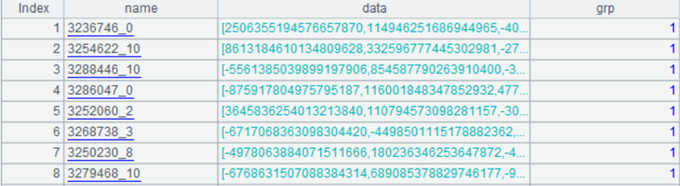
After clustering, two files are outputted: one-member subset data “indexes_1.btx” and multi-member subset data “indexes_m.btx”, both of which have the same data structure in the following form:

The following code is the comparison process implemented in SPL:

	A	B
1	=file(“target_vec.btx”).import@b().run(data=data.i()).i()
2	=sub_no=512
3	=X1=file(“indexes_1.btx”).import@b().run(data=data.i()).i()
4	=X=file(“indexes_m.btx”).import@b().run(data=data.i()).i()
5	=XG=A4.group@v0(grp).(~.run(data=data.i()).i())
6	=A5.(~(1)).run(data=data.i()).i()
7	=(A3|A4).i()
8	=ath_data_num=0
9	=ath_time=0
10	=all_time=0
11	=miss_bit=0
12	for A1	=xx=A12.data.i()
13		=now()
14		=A6.ptop(sub_no;bit1(xx,data))
15		=XG(B14)
16		=B15.conj@v()
17		=B16|X1
18		=B17.minp(bit1(xx,data))
19		=interval@ms(B13,now())
20		=now()
21		=A7.minp(bit1(data,xx))
22		=interval@ms(B20,now())
23		=B18.(bit1(data,xx))
24		=B21.(bit1(data,xx))
25		=ath_data_num+=B17.len()+A6.len()
26		=ath_time+=B19
27		=all_time+=B22
28		=if(B23!=B24,1,0)
29		=miss_bit+=B28
30	=A1.len()
31	=ath_data_num/A30
32	=ath_time/A30
33	=all_time/A30
34	=miss_bit/A30
35	=file(“target_vec.btx”).import@b().run(data=data.i()).i()
36	=sub_no=512

A1: read the target vector data;

A3: read the one-member subset data;

A4: read the multi-member subset data;

A5: group the multi-member sets by grp;

A6: the first member of each subset in A5 is the base vector;

A12 code block refers to the comparison process with each target vector;

B14: select the nearest K subsets;

B18: calculate the nearest members;

B21: traverse all nearest members.

The variables ath_data_num, ath_time, all_time, and miss_hit respectively count the amount of data traversed through algorithm, the time consumed in algorithm, the time consumed in full traversal, and the number of times that the nearest distance calculated through algorithm is not equal to that calculated through full traversal.

A33-A36: the average of the above count result.

We call the ratio that the number of times that the nearest distance calculated through algorithm is not equal to that calculated through full traversal accounts for total number of target vectors (the result in A36) as the miss hit rate. As a measure of algorithm effectiveness, it is clear that the lower the miss hit rate, the higher the algorithm effectiveness.

The following table shows the count result for 10,000 target vectors on the clustering output files “indexes_ 1.btx” and “indexes_m.btx”:

Data amount	Number of subsets traversed	Amount of data traversed through algorithm	Time consumed in algorithm	Time consumed in full traversal	Miss hit rate
900,000	512	80683	2.02ms	18.15ms	5.68%
	1024	114384	3.92ms	17.48ms	2.46%

Mathematical analysis shows that the theoretical complexity of this algorithm is proportional to the square root of data amount, and it takes no more than 100ms to compute tens of millions of data. For example, when the amount of data increases to 90 million, which is equivalent to 100 times 900,000, the time consumed in algorithm only increases by 10 times. To be specific, traversing 512 subsets takes about 20ms, and traversing 1024 subsets takes around 40ms, yet the time consumed in full traversal will be 1800ms, increasing by 100 times.

Stepwise clustering

The above clustering method is to split the whole set into multiple subsets; we call this method split type clustering. This method has a drawback in that it often fails to split data thoroughly. More specifically, the number of subsets has already reached the threshold N when data are not yet split to the extent that the number of members of every subset is less than the threshold M, which will easily result in a situation where the number of members in each subset is not evenly distributed, that is, some subsets have many members, while many subsets have only one member.

In view of this, we design another method called stepwise clustering, and the process is as follows:

Let the member-number threshold of subset be M:

1. The first base vector is the first vector, denoted as _x_1; the first subset is denoted as _X_1;

2. Traverse the whole set X and add its members to the nearest subset Xi (add randomly when the distances are equal);

3. When the number of members added to a certain subset Xi exceeds M, split the traversed data to make the member-number of any Xi is less than or equal to M (the splitting process is the split type clustering process);

4. Loop through steps 2, 3 until X is completely traversed. In order to prevent split type clustering being performed indefinitely, use the formula M’=sqrt (traversed data amount * 1024) to dynamically calculate the subset number threshold based on the amount of data traversed. M’ refers to the threshold for the number of subsets of the traversed data. This ensures the remaining data always has the opportunity to serve as a basis vector.

Compared to the split type clustering, the stepwise clustering can make clustering more thorough, and the final number of subsets is usually smaller.

SPL code for stepwise clustering:

	A	B	C	D	E
1	longdata.btx
2	=s_no=600
3	=file(A1).import@b()
4	=to(A3.len()).psort(rand())
5	=X=A3(A4).new(data).run(data=data.i()).derive@o(:grp,:dis,:new_dis,:flag).i()
6	=G=create(base,num,rad,max_rad_v)
7	=x1=X.data
8	=G.record([A7,0,0,null])
9	for X	=xid=#A9
10		=sub_num_step=sqrt(xid*1024)
11		=v0=A9.data
12		=G.@m(bit1(base,v0))
13		=B12.pmin(~+rand())
14		=B12(B13)
15		=G(B13).run(num=num+1,(dst=B14,flg=dst+rand()>rad+rand(),rad=if(flg,dst,rad)),max_rad_v=if(flg,v0,max_rad_v))
16		=A9.run(B13:grp,B14:dis)
17		=G(B13).num
18		=G.len()
19		if B18>sub_num_step		next
20		if B17>s_no	=X(to(#A9))
21			for	=G.len()
22				if D21>sub_num_step	break
23				=G.groups@m(;maxp(if(num<=s_no||rad==0,-1,rad+rand())):mx).mx
24				if D23.num>s_no	=x1=D23.max_rad_v
25				else	break
26				=G.record([x1])
27				=C20.run@m(bit1(data,x1):new_dis,new_dis-dis<2*rand()-1:flag,if(flag,new_dis,dis):dis,if(flag,D21+1,grp):grp)
28				=D27.groups@nm(grp;count(1):cnt,max(dis):rad,maxp(dis).data:max_rad_v)
29				=G.run@m((rcd=D28(#),num=rcd.cnt,rad=rcd.rad,max_rad_v=rcd.max_rad_v))
30	=A3(A4).derive(X(#).grp:grp,X(#).dis,G(grp).rad:rad)
31	=A30.group(grp)
32	=A31.align@a([false,true],~.len()==1)
33	=A32(2).conj().run(grp=int(grp)).derive(int(#):ID)
34	=A33.len()
35	=A32(1).conj().group([grp,dis]).conj().run(grp=int(grp)).derive(int(A34+#):ID)
36	=file(“indexes2_1.btx”).export@b(A33)
37	=file(“indexes2_m.btx”).export@b(A35)

The inputs and outputs of this algorithm are similar to those of split clustering except for the name.

A4: sort data randomly;

A9 code block refers to the stepwise clustering process;

C21 code block refers to the split type clustering process.

The query process is the same as that of above algorithm and will not be repeated here.

The following table presents the test results of stepwise clustering for the same data:

Data amount	Number of subsets traversed	Amount of data traversed through algorithm	Time consumed in algorithm	Time consumed in full traversal	Miss hit rate
900,000	512	81212	2.33ms	16.63ms	2.43%
	1024	128311	4.37ms	17.20ms	0.82%

The effect is better than that of split type clustering.

Intersection method

From the table above it can be seen that the miss hit rate of traversing 512 subsets is 2.43%, which is still a bit high.

Stepwise clustering is to randomly shuffle all data and then cluster, and it will also randomly handle when meeting equal distances during clustering. Therefore, this method will result in a clustering result with strong randomness. We can utilize the randomness of stepwise clustering to reduce the miss hit rate by taking the intersection of two miss hits after clustering multiple times.

The specific steps are as follows:

1. find the nearest member of each random clustering according to original comparison method;

2. select the closer member from two nearest members (equivalent to taking the intersection of members missed from two clustering results).

The following code is the intersection method implemented in SPL:

	A	B	C
1	=file(“target_vec.btx”).import@b().run(data=data.i()).i()
2	=sub_no=1024
3	indexes2_1_1.btx
4	indexes2_1_2.btx
5	indexes2_m_1.btx
6	indexes2_m_2.btx
7	=[A3:A6].(file(~).import@b(name,data,grp).run(data=data.i()).i())
8	=A7.to(2)
9	=A7.to(3,)
10	=A7.to(3,).(~.group@v0(grp).(~.run(data=data.i()).i()))
11	=A10.(~.(~(1)).run(data=data.i()).i())
12	=(A7(1)|A7(3))
13	=ath_data_num=0
14	=ath_time=0
15	=all_time=0
16	=miss_hit=0
17	for A1	=xx=A17.data.i()
18		=s=0
19		=now()
20		for 2
21			=X1=A8(B20)
22			=X=A9(B20)
23			=XG=A10(B20)
24			=A11(B20)
25			=C24.ptop(sub_no;bit1(xx,data))
26			=XG(C25)
27			=C26.conj@v()
28			=C27|X1
29			=s+=C28.len()+C24.len()
30			=C28.minp(bit1(xx,data))
31			=@|C30
32		=C31.minp(bit1(xx,data))
33		=interval@ms(B19,now())
34		=C31=[]
35		=now()
36		=A12.minp(bit1(data,xx))
37		=interval@ms(B35,now())
38		=B32.(bit1(data,xx))
39		=B36.(bit1(data,xx))
40		=if(B38!=B39,1,0)
41		=ath_time+=B33
42		=all_time+=B37
43		=miss_hit+=B40
44		=ath_data_num+=s
45	=A1.len()
46	=ath_time/A45
47	=all_time/A45
48	=miss_hit/A45
49	=ath_data_num/A45

B20 code block refers to the comparison process of two clustering results.

After clustering twice, comparison should also be made twice during query, and the amount of data traversed is the sum of the data traversed in two comparisons, which will increase comparison time, but it can greatly reduce the miss hit rate.

The following are the test results of random stepwise clustering twice:

Number of subsets traversed	Amount of data traversed	Time consumed in algorithm	Time consumed in full traversal	Miss hit rate
512	163771	6.16ms	16.62ms	0.18%
1024	260452	9.34ms	17.11ms	0.06%

Sort the dimensions

The computation amount can be decreased by reducing the number of dimensions besides the way of reducing the amount of traversed data. If all values on a certain dimension are 0 (or 1), then the contribution of this dimension to the distance is always 0. In other words, the sensitivity of this dimension to distance calculation is 0, so it is obviously unnecessary to calculate the dimension. Similarly, if the majority of values on a certain dimension are 0 (or 1), its contribution to the distance will be much smaller than that of dimension with similar number of 0s and 1s, that is, its sensitivity is lower. Therefore, we give priority to the calculation of dimension with higher sensitivity, and do not calculate dimensions with low sensitivity. In this way, limited computing resources can be fully utilized.

The sensitivity of a dimension is defined as:

1-abs (the number of 1 in the dataset on the dimension/data amount - 0.5)

We sort all dimensions by sensitivity and only calculate the previous part of dimensions to reduce the computing load. We should convert the dimension-sorted binary sequence to long data in the data prepare stage.

Modify the original data conversion process:

	A	B	C
1	=directory@p(“raw_data”)
2	=512*[0]
3	=A1.run(A2=A2++blob(file(~).read@b()))
4	=A1.len()
5	=A2.psort(abs(~/A4-0.5))
6	=func(A12,A1,A5)
7	=directory@p(“x0_data”)
8	=func(A12,A7,A5)
9	=file(“longdata1.btx”).export@b(A6)
10	=file(“div_index1.btx”).export@b(A5)
11	=file(“target_vec1.btx”).export@b(A8)
12	func
13		=A12.group((#-1)\100000)
14		=A12.len()
15		=create(name,data)
16		for B13	=B16.(blob(file(~).read@b())(B12).bits())
17			=B16.(filename@n(~))
18			=C17.(~|[C16(#)]).conj()
19			=B15.record(C18)
20		return B15

A3: count the number of 1s of each dimension;

A5: sort by (1-sensitivity);

A6: convert all data;

A8: convert the target data;

A12 code block is to sort the binary data and convert to long data;

The clustering process is similar to the original one, except that only the previous part of dimensions with high sensitivity are clustered (such as the first p long data, that is, the first p*64 dimensions).

Also, the comparison process is similar, except that:

1. The target vectors need to be sorted by sensitivity before converting to long data. Likewise, take the first p long data;

2. select the topn nearest vectors from the first p long data in the original way. Since only the distances of the first p long data are calculated, it cannot determine that the nearest members of the first p long data are definitely the full-dimension nearest members. Thus, we take the first topn vectors so that there is a high probability to contain full-dimension nearest members. This probability can be further increased by the use of intersection method;

3. calculate the full dimension distances of the topn vectors and find the nearest members;

4. use the intersection method to reduce the miss hit rate.

Test results show that a good miss hit rate can be obtained when p=5 (the first 320 dimensions).

The following code is the comparison process implemented in SPL:

	A	B	C
1	=pre_n_long=5
2	=topn=50
3	=sub_no=1024
4	indexes3_1_1.btx
5	indexes3_1_2.btx
6	indexes3_m_1.btx
7	indexes3_m_2.btx
8	=[A4:A7].(file(~).import@b(name,data,grp).derive(data.to(pre_n_long):data1).run(data=data.i(),data1=data1.i()).i())
9	=A8.to(2)
10	=A8.to(3,)
11	=A8.to(3,).(~.group@v0(grp).(~.run(data=data.i(),data1=data1.i()).i()))
12	=A11.(~.(~(1)).run(data=data.i(),data1=data1.i()).i())
13	=(A8(1)|A8(3))
14	=ath_data_num=0
15	=ath_time=0
16	=all_time=0
17	=miss_hit=0
18	=file(“target_vec1.btx”).import@b()
19	for A18	=xx=A19.data.i()
20		=xx.to(pre_n_long)
21		=s=0
22		=now()
23		for 2
24			=X1=A9(B23)
25			=X=A10(B23)
26			=XG=A11(B23)
27			=A12(B23)
28			=C27.ptop(sub_no;bit1(B20,data1))
29			=XG(C28)
30			=C29.conj@v()
31			=C30|X1
32			=s+=C31.len()+C27.len()
33			=C31.top(topn;bit1(B20,data1))
34			=C33.minp(bit1(xx,data))
35			=@|C34
36		=C35.minp(bit1(xx,data))
37		=interval@ms(B22,now())
38		=C35=[]
39		=now()
40		=A13.minp(bit1(data,xx))
41		=interval@ms(B39,now())
42		=B36.(bit1(data,xx))
43		=B40.(bit1(data,xx))
44		=ath_time+=B37
45		=all_time+=B41
46		=if(B42!=B43,1,0)
47		=miss_hit+=B46
48		=ath_data_num+=s
49	=A18.len()
50	=ath_time/A50
51	=all_time/A50
52	=miss_hit/A50
53	=ath_data_num/A49

B23 code block refers to the comparison process;

C34: calculate the full-dimension nearest distances;

Sorting dimensions decreases the amount of dimension computation and speeds up the clustering calculation a lot.

The following table is the comparison results of stepwise clustering, intersection method, and sorting dimensions for the data of 900,000:

Data amount	Number of subsets traversed	Amount of data traversed	Time consumed in algorithm	Time consumed in full traversal	Miss hit rate
900,000	512	159381	5.60ms	17.46ms	0.68%

The algorithm performance is improved by about 10%.