The association calculation in SPL differs significantly from that in SQL. SQL defines join as an operation that first calculates the Cartesian product and then filters. SPL also provides this operation, yet it has better alternatives in most scenarios, so this operation is not recommended.

Programming in SPL to implement association calculation needs to subdivide join into different types first, and then select the corresponding function to code.

Classification of association calculations

The equivalence JOIN in the figure refers to the join whose filter condition is that the field of one table is equal to the corresponding field of associated table. In practice, the non-equivalence JOIN is rare and most of such joins can be converted to equivalence join. Therefore, we mainly focus on the equivalence join in this article.

Equivalence join includes three types: foreign key join, primary key join, and other join.

The foreign key join refers to the equivalence join between a certain field of table A and the primary key of table B. Table A is called the fact table and table B is called the dimension table; the field in table A that associates with the primary key of table B is called the foreign key that A points to B, and B is called the foreign key table of A.

The primary key join refers to the equivalence join between the primary key of table A and the primary key or part of primary keys of table B.

Both of the above joins involve primary key, which is not necessarily a physical primary key and can also be a logical primary key.

The ‘other JOIN’ in the figure refers to the equivalence join that doesn’t involve primary key and usually appears only when an error in business logic or data occurs.

The primary key join can be subdivided into homo-dimension join and primary-sub join. The association between the primary key of table A and the primary key of table B is called the homo-dimension join, and A and B are mutually referred to as homo-dimension table. The association between the primary key of table A and part of the primary keys of table B is called the primary-sub join, and A is called the primary table and B is called the sub table.

The three types of joins in the figure, including the foreign key JOIN, homo-dimension JOIN and primary-sub JOIN, cover the vast majority of equivalence join scenarios, and it can be said that almost all equivalence joins with business significance fall into the three joins. Limiting equivalence join to the three joins will hardly reduce its scope of application.

SPL provides different functions for foreign key join and primary key join. When performing join operation, we first need to determine the type of join and identify the primary key involved.

If the data volume of the tables to be associated is not large and can be loaded into memory, such join is called the in-memory join. This article will focus primarily on the programming method of in-memory join.

Foreign key join

Take the join between the order table and the employee table as an example:

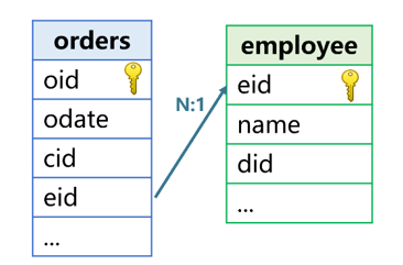
The employee field ‘eid’ of the orders is associated with the primary key field of the employee; the orders is a fact table and the employee is a dimension table.

The eid of orders is the foreign key that the orders points to employee; the employee is the foreign key table of orders; the Orders and the employee are in a many-to-one relationship. Other fields include the order date (odate), customer number (cid), employee name (name), and employee department number (did).

The purpose of performing foreign key join on two tables is to utilize both the fields of fact table and the corresponding fields of dimension table during calculation. For example, the name field of employee and the odate field of orders will be utilized when filtering the order data by employee name and order date.

T.switch function

On the premise that both the fact table and the dimension table can be loaded into memory, the T.switch function will convert the foreign key field of T table (fact table) to the address of the corresponding dimension table record, allowing us to directly reference the field of dimension table record through the address during calculation. This method is called foreign key addressization.

With this method we can convert the eid field of orders to one record of employee, and the name field in this record can be referenced through eid.name during calculation. The “dot operator” in the function refers to the address reference. In this way, the code to filter the order data by employee name and order date will be:

	A	B
1	=file("employee.btx").import@b().keys(eid)	=file("orders.btx").import@b()
2	>B1.switch(eid,A1:eid)
3	=B1.select(eid.name=="Tom" && odate=…)

A1 is to read the employee into memory and define its primary key as eid; B1 is to read the orders into memory;

A2 is to convert the eid field of orders to the address of the corresponding record in employee, which is the process of foreign key addressization. Because the primary key of employee is already determined as eid, A2 can be simplified as orders.switch (eid, A1).

In A3, the name field of employee can be referenced naturally through eid.

After being processed by T.switch, we will feel that the records of the two tables are really associated, and that the field value of fact table T is the record of dimension table, allowing us to reference corresponding field of dimension table through the field of fact table.

According to the definition of SPL on foreign key association, the associated field of dimension table must be the primary key, then the dimension table record associated with the foreign key field of each record in fact table is unique. In other words, the eid field of each record in orders will associate with unique record in employee. This ensures each record in orders has unique eid.name value, which can be clearly defined. By virtue of this unique function, SPL implements foreign key addressization.

Implementing multi-level foreign key join with T.switch

A fact table usually corresponds to multiple dimension tables, and dimension tables may be in many levels. In this case, the advantage of foreign key addressization in coding can be more clearly demonstrated. Take the figure below as an example:

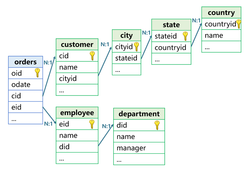
For such foreign key association with multiple or multi-level dimension tables, foreign key addressization can be done one by one. The customer number field ‘cid’ of orders is the address of the record in the customer, and the cityid field of customer is the address of the record in the city, and so on and so forth. In this way, the name of the country where the customer corresponding to a certain order is located can be written as cid.cityid.stateid.countryid.name, and the name of the department where an employee belongs to can be written as eid.did.name.

Such coding method greatly simplifies the code. Let’s illustrate this through an example. Suppose that, for orders that the country where the customers are located is “US” and the department that the employees belong to is “Sales”, we want to group the orders and count the number of orders by the state and city where the customers are located, then the SPL code will be:

	A	B
1	>state.switch(countryid,country)	>city.switch(stateid,state)
2	>customer.switch(cityid,city)
3	>employee.switch(departmentid,department)
4	>orders.switch(cid,customer;eid,employee)
5	=orders.select(cid.cityid.stateid.countryid.name=="US" && eid.did.name=="Sales")
6	=A5.groups(cid.cityid.stateid,cid.cityid;count(1))

Here we omit the code for reading tables, defining primary key and assigning the value to corresponding variable, such as:

>country=file("country.btx").import@b().keys(cid)

A1 utilizes the T.switch function to convert the countryid field in the state to the address of record in the country. This allows us to reference the field in country through the countryid filed, hereby implementing the foreign key addressization of country.

B1 converts the stateid field in the city to one record in the state, thus implementing the addressization of multi-level foreign keys of three tables ‘city, state and country’.

A2 to A3 implement the addressization of multi-level foreign key of four tables such as the customer and two tables such as employee in sequence.

In A4, the orders has two foreign keys, and the T.switch function can convert them to the addresses of records in two tables simultaneously.

A1 through A4 can be regarded as the preparation stage for foreign key addressization. Once the preparation is accomplished, we can write the filter condition and the grouping expression naturally in A5 and A6.

More importantly, the primary key and foreign key of tables are usually already determined, and any table that has undergone foreign key addressization can be reused. When calculating, we can just code like A5 and A6, which is very convenient. We can perform foreign key addressization following the read of data table into memory when the system starts, this action is called pre-association.

Usually, the value of foreign key field will surely be within the range of the primary key values of dimension table. However, there may be exceptions. For example, when a new employee is not yet assigned to a department, the ‘did’ field will be filled with 0, which will result in a situation where there is no corresponding record in the department. In this case, we can use different options of T.switch function to obtain different desired results.

	A	B
1	=file("department.btx").import@b().keys(eid)	=file("emplopyee.btx").import@b()
2	=B1.switch(did,A1)	=A2.count(did.name==null)
2	=B1.switch@i(did,A1)	=A2.count(did.name==null)
2	=B1.switch@d(did,A1)	=A2.count(did.name==null)

Note that there are three consecutive line numbers ‘2’ in this code, which means the three lines of code are to be executed separately rather than sequentially. This is because B1 will be changed after execution, and if A2 changed, the desired result would not be obtained.

T.switch without any option will fill the foreign key with null when the dimension table record corresponding to the foreign key is not found, and it will not report an error when referencing the field again, and will return null only. Therefore, for the employee record whose did is originally 0 in A2, the did field will be converted to null. And correspondingly, B2 will be the number of records whose did originally being 0.

T.switch@i will delete the fact table record that fails to find corresponding foreign key record to ensure any foreign key of fact table is correctly converted to dimension table record. Therefore, the employee whose did is originally 0 in A2 will be deleted, and accordingly, the number of records in B2 will be 0.

T.switch@d will retain only the fact table record that fails to find corresponding foreign key record, and cannot convert foreign key any more. In other words, the employee whose did is originally not 0 in A2 will be deleted, and the did of retained record will not be converted and will still be 0. As a result, B5 will report an error because the value 0 is not an address and the “dot operator” cannot be utilized.

T.join function

In certain scenarios, some values of foreign key field of a fact table may have no corresponding record in dimension table. In this case, T.switch function will convert foreign key to null, which will result in the loss of the original foreign key value.

For example, the department numbers of some employee records are written incorrectly, resulting in a failure to find corresponding department. In this case, when using T.switch to associate the employee table with the department table, the department number field ‘did’ of such employee records will become null. If the original foreign key value must be retained, we can use the T.join function to join certain fields of dimension table onto the fact table T. For example, the code to join the department name field and the manager field onto the employee is:

	A
1	=employee.join(did,department,name:dname,manager:dmanager)

A1 creates a new table, which contains all fields of the employee, as well as the name and manager fields of the department.

The parameters of T.join include, in turn, did (the foreign key), department (the dimension table), name (the field of dimension table, to be renamed as dname), and manager (the field of dimension table, to be renamed as dmanager).

We can also assign the addresses of dimension table records as a new field and join them onto the fact table with the T.join function, which can not only implement foreign key addressization but also avoid the loss of foreign key field value mentioned above. For example, for the employee table and department table, the code to query the employees who belong to the department “Sales” is:

	A
1	=employee.join(did,department,~:did_fk)
2	=A1.select(did_fk.name=="Sales")

A1 creates a new table. In addition to the fields of the employee, a new field ‘did_fk’ is added to store the addresses of the corresponding records in the department. If no corresponding record is found, it will be filled with null. This is equivalent to making a copy of the foreign key field ‘did’ and accomplishing foreign key addressization.

A2 uses the did_fk to reference the name field of the department.

Unlike T.switch function, T.join function does not directly convert the fields of original table, but generates a new table. Therefore, attention should be given to the order when performing the addressization of multi-level foreign key. For the data table that serves as both fact table and dimension table, it needs to associate its own dimension table first to obtain a new data table, and then associates with the fact table.

Implementing multi-field association with T.join

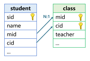
T.switch function does not support the situation that multiple fields are served as the primary key of dimension table and the foreign key of fact table. To solve this, we also need to employ the T.join function. Assume the two fields, major number and class number, are the foreign keys that the student table points to the class table, as shown in the following figure:

The code to join the teacher field onto the student table with the T.join function is:

	A
1	>class.keys(mid,cid)
2	=student.join(mid:cid,class,teacher)

A1 defines two primary keys for the class table. A2 creates a new table based on the student table, adds the ‘teacher’ field of class table, fills it with the class teacher. The first parameter ‘mid:cid’ of the T.join function represents two associated fields, which should be separated by a colon.

Like the T.switch function, T.join also provides the @i and @d options to handle the situation where the foreign key value cannot be found in dimension table. Still, let’s take the case where a new employee whose did is 0 and no record is found in the department table as an example:

	A	B
1	=file("department.btx").import@b().keys(eid)	=file("emplopyee.btx").import@b()
2	=B1.join(did,A1,name:dname)	=A2.count(dname==null)
3	=B1.join@i(did,A1,name:dname)	=A3.count(dname==null)
4	=B1.join@d(did,A1)	=A4.count(dname==null)

Note that A2, A3 and A4 can be executed sequentially. This is because T.join is to generate a new table, and B1 will not change after execution, and execution can continue.

T.join without any option will make the value of new field dname become null for the employee record whose did is originally 0 in A2. And correspondingly, B2 will be the number of records whose did originally being 0.

T.join@i will delete the employee record whose did is originally 0 in A3. And accordingly, the number of records in B3 will be 0.

T.join@d will delete the employee record whose did is originally not 0 in A4. The @d option requires that there is no the parameter name:dname, otherwise it will be invalid, and the calculation result is the same as that without @d option. Correspondingly, an error will be reported in B4 because the result does not contain dname field.

Primary key join

Homo-dimension join

The join between the employee table and the manager table is a homo-dimension join:

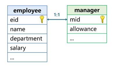
Because some employees themselves are manager, and manager has more attributes than common employees such as post allowance, a separate manager table needs to be created. The primary key ‘eid’ of employee is associated with the primary key ‘mid’ of manager, and the values of the two fields are both employee number.

join function

The join function and the above T.join are two different functions. Let’s first look at the usage of join function and then explain the differences.

Suppose we want to query the number, name and total income (salary + allowance) of every employee (including managers), the code will be:

	A	B
1	=file("employee.btx").import@b().keys(eid)	=file("manager.btx").import@b().keys(mid)
2	=join@1(A1:e,eid;B1:m,mid)
3	=A2.new(e.eid:eid,e.name:name,e.salary+m.allowance:income)

The join function in A2 will return a new table with two fields, e and m. This function will join the employee records in A1 with the manager records in B1, that is, it will fill in the ‘e’ and ‘m’ fields of the new table respectively with the addresses of the records where eid and mid are equal, serving as one record of new table. The @1 option of join function will be explained later.

The value of ‘e’ and ‘m’ fields is the address of record, somewhat like the result of foreign key being converted by T.switch function.

Because both tables have defined their own primary key, A2 can be simplified as: =join@1(A1:e;A2:m).

A3 utilizes the result of A2 to generate a new table containing three fields: eid, name, and income. Since the values of both the ‘e’ and ‘m’ are records, we can use ‘e’ to reference employee number, fill in the name field with the eid and name fields of new table, and use the employee salary plus the manager allowance field referenced by m to get the income field of new table.

This code uses the two fields ‘e’ and ‘m’ of new table created in A2 to reference the fields of the tables in A1 and B1 respectively, which is natural and easy to understand just like foreign key addressization.

In this example, the employee table contains manager, but not every employee is manager. In other words, many employees do not have corresponding records in the manager table. To solve this, the ‘m’ field of new table will be filled with null, so that their total income is equal to their respective salary.

In this case, join@1 will take the table on the left (the first parameter of join function) as base table to associate the other table. If there is a record in the other table that is the same as the record of association field of the left table, the two records will be associated. Otherwise, a null will be filled in. This type of join, which takes the first table on the left as base table, is called the left join. @1 means the number 1, not the letter I, indicating that the association is performed based on the first table. Since the tables in homo-dimension relationship are associated through primary key, the values of association field of generated table sequence are the same as those of the left table, and the length is also the same as that of the left table. When associating three or more tables by the way of left join, the leftmost table is also taken as the reference table.

SPL does not provide right join, because we only need to change the position of the parameters of function.

Homo-dimension join is also applicable to instantly generated tables, as long as the fields to be associated are primary key. For example, the contract table, payment table, and invoice table:

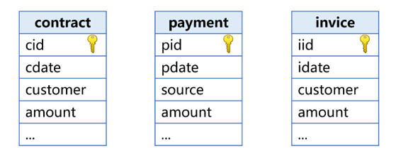
Now we want to count the contract amount, payment amount and invoice amount of each day. To solve this problem, we can group the three tables respectively by date and aggregate respective amount, and regard the results as three tables. Due to the fact that the grouping field ‘date’ is unique, date naturally becomes the primary key of the three tables. The three tables have the same primary key, which meets the definition of homo-dimension table. Associating the three tables by the primary key (date) is a homo-dimension join. Therefore, this problem can be solved with join function, the code is:

	A	B
1	=file("contract.btx").import@b()	=A1.groups(cdate;sum(amount):amount)
2	=file("payment.btx").import@b()	=A2.groups(pdate;sum(amount):amount)
3	=file("invice.btx").import@b()	=A3.groups(idate;sum(amount):amount)
4	=join@f(B1:c;B2:p;B3:i)
5	=A4.new(ifn(c.cdate,p.pdate,i.idate):adate,c.amount:camount,p.amount:pamount,i.amount:iamount)

A1 to B3: aggregate the respective amount of three tables by date in sequence. The aggregated results in B1, B2, and B3 are tables with date as the primary key;

A4: associate B1, B2, and B3 to generate a new table whose three fields, c, p, and i, store the records of B1, B2, and B3 respectively;

A5: utilize A4 to reference the fields of three tables and generate another new table to get desired results.

From the perspective of requirements, the date where the contract amount, payment amount and invoice amount are all null won’t appear in the result. However, as long as one of the amounts isn’t the null it should be put in the result. The join@f used in A4 will take into account all tables to be associated. As long as the value of the association field exists in any of the tables, a record will be generated in the result table, and the record of the table that has the value will be filled in the corresponding field to implement association, and the value of field that does not has the value will be filled with null. The set of remained association field values in the final result table will be the union of the association field sets of multiple table sequences participating in association. This type of join that takes all tables into account is called full join.

Because any field c, p, and i may be null in the result of full join, A5 needs to use the ifn function to return the date field of the first non-null record among the three records, using as the date field of the final result.

Primary-sub table

A typical example of primary-sub table is the order table and the order detail table, as shown as below:

The primary keys of the order detail table are the order number ‘oid’ and the product number ‘pid’. The primary key ‘oid’ of order table is associated with part of primary keys ‘oid’ of the detail table. The order table is the primary table and the order detail table is the sub table, they are in one-to-many relationship.

When associating the tables in primary-sub relationship, SPL also uses the join function. For example, we want to calculate the total order amount of each customer, the code is:

	A	B
1	=file("orders.btx").import@b()	=file("order_detail.btx").import@b()
2	=join(A1:o,oid;B1:od,oid)
3	=A2.groups(o.cid:cid;sum(od.price*od.quantity))

The join function in A2 will join the order records in A1 with the detail records in B1, that is, the records with equal oid are filled in the ‘o’ and ‘od’ fields respectively, serving as one new record in the new table.

Unlike the homo-dimension join, the oid is only one of the primary keys of detail table, and there may be multiple records with the same oid in the detail table. In this case, the result of join function will contain duplicate order record, with each detail record being associated with one order record, and each order record being associated with multiple detail records. As a result, the number of records is the same as that in detail table.

The join function without any options will find out the records of the association fields of all tables that exist and are equal and associate them. If a record of the association field of a certain table does not exist in any other table, this record will be discarded. This type of join is called the inner join.

join function and T.join function

The definition, computing method, coding way, and applicable scenario of join are all different from those of T.join.

In SPL, two data tables are associated in such a way that generates a new data table with two fields through the equality relationship of a certain field (or expression), and makes the two fields of new table respectively correspond to the addresses of the corresponding records of the two data tables. Such association operation is called join, the field (or expression) used to determine association is called association key, and the records with equal association key value are called the associated record.

SPL uses the join function to implement join.

Foreign key join is also a kind of join operation, which utilizes the foreign key of fact table and the primary key of dimension table as the association key.

In fact, the T.join function also uses a similar way as the join function to associate the records of fact table and dimension table, and generates a new table by utilizing the fields of fact table, and the referenced fields of the corresponding records of dimension table.

The reason why SPL provides T.join function is that the calculation that combines join and field reference is more common and more convenient for foreign key join.