What is a time key?

While relatively stable, the data of dimension table may still change. For example, the city where a certain customer is located changed from New York to Chicago on May 15, 2020.

When associating the order table with customer table, the order before this date should be associated with the old customer record (that is, the city should still be New York), while the order on and after this date should be associated with the new customer record (that is, the city should be Chicago).

In other words, we need to find the correct customer record for each order, i.e., the latest customer record when the order is generated (order date).

In relational databases, the snapshot or slowly changing dimensions (SCDs) is often used to meet the data change requirement of dimension table. However, this method will cause problems such as making the calculation complex, occupying more storage space.

To solve such problems, SPL adds a special primary key called the time key in addition to common primary key. The data of time key are all the time or date type data, and will be specially processed when querying by primary key, which can effectively solve the problems caused by data change of dimension table.

Correspondingly, we call the common primary key the basic key.

For example, the following customer table is added with a time key (effective time of record: ‘edate’ field):

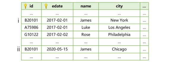
This customer table has two primary key fields, customer number ‘id’ and effective time of the record, of which the second is the time key. Since the city where customer B20101 is located changed on 2020-05-15, there are two different records respectively in the edate and city fields.

Now we want to query the latest customer record by a specified date, the code of using the time key is roughly as follows:

	A	B
1	=T("customer.btx")	>A1.keys@t(cid,edate)
2	=A1.find('B20101',date(2020-05-01))
3	=A1.pfind('B20101')

A1: read the customer table; B1: define two primary keys cid and edate. The @t option represents that the last primary key field edate is the time key, and cid is the basic key.

If business requires, we can also use a date/time type field with higher precision (such as seconds or milliseconds) as the time key.

A2: search for records by the specified customer and date. The records found by cid are not unique, and SPL will then search them for the record whose time key is no greater than and closest to 2020-05-01, which refer to the record whose city is New York here.

We can see that searching by time key is not an equivalence search, but a search for record that are no greater than and closest to the specified time.

A3: search for the sequence number position of record by the specified customer and time. The time parameter is omitted here. SPL will automatically take the current time as the time key parameter to search for the latest record as of the current time, and will return the sequence number of record whose city is Chicago.

Time key in foreign key association

After adding the time key to a customer table (dimension table) and associating the customer table with order table (fact table) on the customer number ‘o_cid’ of order table, a situation may arise where multiple records of customer table are found for each order of o_cid. In this case, it needs to find out the records whose effective date ‘edate’ is not greater than and closest to the order date ‘odate’ from the found records.

In other words, the date fields of the two tables are not in an equivalence relationship, making it impossible to perform an equivalence association between the customer number and order date of order table and the customer number and effective date of customer table.

When a dimension table is small and can be stored entirely in memory, we can utilize the table sequence with a time key to store the dimension table. The time key is created on the index of table sequence, switch/join supports foreign key association calculation on dimension table with a time key. Alternatively, we can write the find expression to fjoin function to implement such calculation. The code is roughly as follows:

	A	B
1	=file("customer.btx").import@b(cid,edate,city)	>A1.keys@t(cid,edate)
2	=file("orders.ctx").open().cursor(o_cid,odate,amt)
3	=A2.fjoin(A1.find(o_cid,odate),city)
4	=B2.groups(city;sum(amt),count(~))

A1: read the customer table. B1: define two primary keys id and edate, and the last primary key edate is the time key;

A2: create a cursor for the order table;

A3: associate the cursor with the customer table in A1. The association fields of order table are o_cid and odate, and the primary keys of customer table are cid and edate.

At this point, in addition to searching for cid equal to o_cid, the find function will also compare the transaction time ‘odate’ with ‘edate’ to find out the edate value that is not greater than and closest to odate. The record where the found value is located is the corresponding association record, that is, the latest customer record as of odate.

A4: use the associated result cursor to group and aggregate the transaction amount and transaction times by city where the customer is located. At this time, there is no need to pay attention to the time key.

Suppose we want to filter out records that cannot be associated with both the fact table and dimension table, we can use fjoin@i. In this case, if the fact table is a composite table cursor, it is recommended to employ the composite table cursor association and filtering mechanism to implement foreign key association and filtering as it can achieve better performance. The code is roughly as follows:

	A	B
1	=file("customer.btx").import@b(cid,edate,city)	>A1.keys@t(cid,edate)
2	=file("orders.ctx").open().cursor(o_cid,odate,amt; o_cid=A1.find(o_cid,odate))
3	=B2.groups(o_cid.city;sum(amt),count(~))

A2: write the original expression in fjoin in the pre-cursor filter condition. The find function will assign the found dimension table record to o_cid, and filter out the orders for which no records are found;

A3: now o_cid can reference the field of dimension table through the dot operator “.”;

The filter expression in A2 is executed before the generation of order record, and the order record that does not meet condition will not be generated. This is why the performance of the above-mentioned mechanism is better than that of fjoin@i. For details, visit: New association calculation methods of SPL .

Time key in primary key association

The switch/join/fjoin function can implement association between the fact table and dimension table (with a time key), but it requires the dimension table to be fully loaded in memory. If a dimension table is so large that it needs to be stored to external storage, these functions cannot be used. Currently, SPL does not provide the time key mechanism for dimension table in external storage.

We know that when a primary table is associated with a sub table, the primary table can be regarded as the dimension table of the sub table. Likewise, this primary table may also face the time key problem.

For example, when we use the customer number and order number as the primary keys of order table, the customer table and order table are in the primary-sub relationship. If the data in the primary table changes, for example, the city where the customer is located changes, it needs to find the latest customer data generated at the time of order generation (order date) for each sub-table record (order).

In this case, SPL allows the creation of a time key on the primary table served as a dimension table, and uses pjoin to perform the external storage primary-sub association involving time key.

Note: join/joinx does not support such primary key association.

The steps to implement such association are as follows: store the primary table (customer table) and sub table (order table) as composite table, then define the time key “effective time of record ‘edate’” on the primary table, and finally use pjoin to implement primary-sub association.

The code of generating composite table is:

	A
1	…
2	…
3	=file(“customer.ctx”).create@t(#cid,#edate,city,…)
4	=file(“orders.ctx”).create(#o_cid,#odate,oid,amount,…)
5	=A3.append(A1)
6	=A4.append(A2)

A1, A2: sort both the customer data and order data by customer number and date in preparation for reading them from data source, which is equivalent to a sortx calculation;

A3: create@t means the dimensions (#cid, #edate) are used as primary key, and the last key edate is the time key;

A4: use the customer number and order date of order table as dimension, indicating that the data is ordered by these two fields.

Once the data is prepared, association can be implemented with the following code:

	A
1	=file("customer.ctx").open().cursor(cid,edate,city)
2	=file("orders.ctx").open().cursor(o_cid,odate,amount)
3	=A2.pjoin@t(o_cid:odate,amount;A1,cid:edate,city)
4	=A4.groups(city;sum(amount))

A1: SPL will automatically discover the time key ‘edate’ on the customer composite table;

A3: appending the @t option to pjoin will automatically process the time key on the table in A1 during calculating.

In other words, each record of o_cid in the sub table (order table) may correspond to multiple records of primary table (customer table), from which SPL will automatically find the record of edate that is not greater than and closest to odate, which is the latest customer record corresponding to the order.

Since the order and customer are in many-to-one relationship, one customer record will be duplicated multiple times according to the number of the corresponding order record, hereby implementing association with these order records.

The pjoin function only supports the situation where the sub table is associated with primary table, and the primary table has a time key. In fact, the primary table in this situation is equivalent to a dimension table, and what pjoin solves is still the problem of dimension table data change.