Routine for real-time data appending (zone table)

Background and method

This routine is applicable to the following scenarios: the real-time requirement for data maintenance is very high, the cycle period for appending data is short, and data may be appended at any time; the data need to be stored in multiple zone tables (hereinafter referred to as ‘table’ unless otherwise specified) of a multi-zone composite table in layers; only the append mode is supported, and the data appended at a time is relatively small and can be stored in a table sequence.

Method:

1. In order to meet the requirement of such scenarios where the append period is too short to accomplish data merge, we store the data in layers. Specifically, write new data quickly to the buffer, and then use another thread to regularly write the buffer data to the recent small-segmentation-interval tables. Since such tables are small, data merge can be quickly accomplished within the append period.

2. Use the merge thread to merge the small-segmentation-interval tables into a larger-segmentation-interval table. After merge, we can query the new larger table and delete the original small tables. The segmentation interval can be divided into multiple layers, and the data can be merged upwards layer by layer. We should strike a balance between the number of segments (which affects read performance) and the interval size (which affects merge performance).

For example, the data can be divided into three layers: day, hour, and minute. We can store the data of every 10 minutes to one table, and merge six tables into an hour table at the end of an hour, and merge the 24 hour tables into a day table at the end of a day. On a new day, continue to generate new hour tables. The whole data is in a multi-zone composite table composed of the day table of previous day, the hour tables of the current day, and the minute tables of the current hour.

When querying, select the table number that meets the time period requirement based on the time period parameter and return, so as to generate a multi-zone composite table for query.

Definitions and concepts

1. Write the new data to the buffer as soon as it is received, and the buffer files are identified and named after the time that data are passed in; write the buffer data to the table of layer 0 in the write-out thread, delete the processed buffer file, and write the remaining data to a new buffer file.

2. Set the chaos period parameter. The vast majority of data would be appended in the chaos period; we should allow appending the data generated before chaos period at low frequency; the data in chaos period should not be written out and participated in calculations.

3. Write out the data in multi-zone composite table format. The multi-zone composite table consists of multiple tables, with each table containing the data of a time interval.

4. Store the data in layers by time, with layer 0 storing the data written directly from the buffer, and layer n storing the data merged from layer n-1.

5. Except for layer 0, each layer has a time level. Now, only four levels are supported: day, hour, minute, and second, and the time levels of different layers cannot be the same.

6. Store data to a new table after every corresponding specified number of layer-level time, and the time interval to which the table corresponds is called the layer interval; the upper-layer interval would be divided into multiple (integer) lower-layer intervals, and the time unit of layer interval is the layer level.

7. Merge mode: merging the data of layer n-1 to layer n is batch merge: there may be multiple tables at a certain layer, and each interval corresponds to one table; once the tables of lower-layer interval that corresponds to the upper-layer interval are all ready, merge them to the table of upper-layer interval.

8. Last table number: each layer has a last table number, which is not a physical table number but the layer n table number calculated based on previous merge (current time - chaos period). The current merge is initiated only when the layer n table number calculated based on (current time - chaos period) is greater than the last table number recorded last time, which can ensure the merge time point of each layer is predesigned, and avoid frequent merges.

9. Month accumulation: if the day layer is the highest layer, it can be directly accumulated as a month table, that is, it can be directly named after the month table number, yet the maximum table number is still the day table number.

10. Write-out thread: execute this thread regularly based on the chaos period to write the data before the chaos period in the buffer to layer 0 tables;

11. Merge thread: from layer 0, merge the tables of each layer n-1 into layer n.

12. Query thread: select the table number that meets the time period requirement based on the time period parameter and return, so as to generate a multi-zone composite table for query.

13. Rule for calculating table number: name it with the starting point of the time interval of data in the table. The number of binary bits corresponding to each time component: year (4) + month (4) + day (5) + hour (5) + minute (6) + second (6) + layer 0 (1) = 31, where the value of layer 0 is the fixed value 1; the hour, minute, and second components are all added with 1, meaning that any component is calculated starting from 1. For the upper-layer table number, set the value of all binary bits on the right to 0 based on the layer level, and divide the value of the current layer level by the layer interval and then add 1.

14. The table number at the highest layer is in plain text. If it involves year and month, the format is yyMM00k; if it involves year, month, and day, the format is yyMMddk, where k is an alternate bit with a value of 0 or 1.

15. Alternate bit: if the target table exists, merge the table and the data merged from lower layer together and write to a new table. The last binary bit of the new and old table numbers alternates between 0 and 1. For example, when the last bit of the original target table number is 0, that of the new table number is 1, and vice versa. Moreover, all the previous bits of new table number have the same value as those of the original target table number.

16. Query period: set the maximum query period. At the end of the merge operation, write the merged table number to the discard table number list and record the discard time, and delete it from the list. Only when the length of discard time exceeds the max query period can such tables be deleted from the hard disk and discard list. This mechanism ensures that a merged table, if being queried, will not be immediately deleted, thus avoiding query error.

Configuration file description

Configuration file: ubc.json

By default, this file is located in the main path of esProc (if you want to save it to another directory, modify the code to use an absolute path). The configuration file includes the following contents:

[{ "choasPeriod":10,
"sortKey":"account,tdate",
"timeField":"tdate",
"otherFields":"ColName1,ColName2",
"bufferDir":"buffer/",
"buffer":[],
"dataDir":"data/",
"dataFilename":"data.ctx",
"queryPeriod":120,
"level":[0,1,2,3,4] ,
"blockSize":[65536,131072,262144,524288,1048576],
"interval":[60,10,2,1],
"lastZone":[null,null,null,null],
"monthCumulate":true,
"discardZone":[],
"discardTime":[]
}]

“choasPeriod” refers to the time length of chaos period, which is an integer measured in seconds.

"sortKey” refers to the sorting field name, and generally includes the time field. When there are multiple such fields, they are separated by commas.

“timeField” refers to the name of time field.

“otherFields” refers to the name of other fields. If there are multiple other fields, separate them by commas.

“bufferDir” refers to the storage path of buffer backup file relative to the main directory.

“buffer” refers to the list of buffer backup file names, and is initially filled with [] and thereafter calculated automatically by program.

“dataDir” refers to the storage path of table relative to the main directory.

“dataFilename” refers to the name of composite table file, such as “data.ctx”.

“queryPeriod” refers to the maximum query period measured in seconds. When a certain table has been discarded for a length of time longer than this period, the table will be deleted from the hard disk.

“level” refers to the layer level, and its values are 0, 1, 2, 3, and 4, representing the layers 0, second, minute, hour, and day respectively. Except for layer 0, other layers can be selectively configured but must be in an order from small to large. For example, the layers can be configured as [0,3,4], yet we cannot configure the layers as [0,2,1,3,4] because it is out of order, nor can we configure layers as [1,2,3,4] because layer 0 is missing.

“blockSize” refers to the block size set for the table of each layer. Generally, set the min block size as 65536 and set the max block size as 1048576; setting it too small or too large is inappropriate. The block size is the size of one block that needs to be expanded each time if the table capacity is not enough when appending data to it. When reading the table data, only one data block can be read at a time, regardless of how much actual data is in the table. However, the table is stored by column and block, with at least two blocks required to store a field - one block is used to store the block information, and the other is used to store data. Therefore, when the number of fields in a table is very large, and many fields need to be read when reading data, the memory space required is [number of fields read * 2 block size]. The smaller the block is set, the less memory space it takes up. But if the amount of data is very large, the larger the block is set, the faster the data will be read. Therefore, for low-level tables, we can set a smaller block size to save memory space; for high-level tables, we can set a larger block size to speed up data reading due to the larger amount of data.

“interval” refers to the layer interval, i.e., the time length in units of layer level. There is no interval for layer 0, and the value of day layer can only be filled with 1, and other layers should be filled based on actual needs. The parameter filled in can only be an integer. Fill the first one in layer 1, and fill the second one in layer 2. The number of parameters filled in is one less than that of levels because there is no value of layer 0.

“lastZone” refers to the last table number of each layer. Since layer 0 has no this parameter, the number of table numbers will be one less than that of levels; all such table numbers are initially filled with null.

“monthCumulate” refers to whether or not to accumulate as monthly table.

“discardZone” refers to the list of the discarded table numbers, the content of which is automatically generated by code, and is initially set as [].

“discardTime” refers to the discarded time list, the content of which is automatically generated by code, and is initially set as [].

Storage structure

1. Data structure of buffer

It is the arrangement composed of data passed in by the user, which retains user’s original data structure.

2. Storage directory and naming rule for data file

Files and sub-paths in the main path:

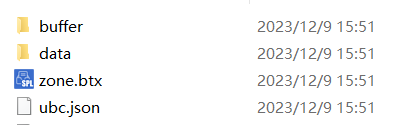
buffer: refers to the storage path of buffer backup file, and the directory name is set in ubc.json (refer to the description above).

data: refers to the storage path of composite table, and the directory name is set in ubc.json (refer to the description above).

zone.btx: refers to the file used to store the table numbers at all levels.

ubc.json: refers to configuration file.

The buffer backup file is named after its read time, and the name format is ‘yyyyMMddHHmmss.btx’.

The files under ‘data’ include:

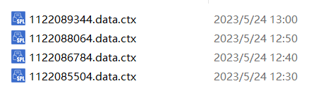
The form of file name is ‘table number.composite table file name.ctx’, where the composite table file name can be set in ubc.json (refer to the description above), and the table number is automatically calculated by the system based on the layer level (see section 2 for the rule for calculating table number).

Configuration and storage examples

1. e-commerce system

Number of users: 100 - 10 million; number of records per day: 1 million - 5 million rows; chaos period: 10 minutes.

In this example, since the data amount is small and the chaos period is long, setting up two layers would be enough. Specifically, set the first layer as 2 hours and set the second layer as 1 day; set the month accumulation as true; directly accumulate the highest-layer data as monthly table. By configuring in this way, it can avoid generating too many tables.

The configuration file is as follows;

[{ "choasPeriod":600,
"sortKey":"uid,etime",
"timeField":"etime",
"otherFields":"eventID,eventType",
"bufferDir":"buffer/",
"buffer":[],
"dataDir":"data/",
"dataFilename":"data.ctx",
"queryPeriod":600,
"level":[0,3,4],
"interval":[2,1],
"lastZone":[null,null],
"monthCumulate":true,
"discardZone":[],
"discardTime":[]
}]

2. Signal system

The characteristics of this system include: i)high data generation frequency (each monitoring point generates multiple pieces of data within one second); ii)rely heavily on the collection time (it is required that each piece of data corresponds to a unique time); iii)many monitoring points and large data amount (a conventional real-time monitoring system usually has thousands upon thousands of monitoring points; each point generates data every second, and dozens of GBs or more data are generated every day). The number of device IDs or monitoring point names is 1-100,000, and the number of records is appended once per second. We can set a 10-second chaos period, the data amount per day is approximately 1.7 billion rows.

In this example, since the data amount is very large (over 1 million rows of data are generated per minute), we set the time interval of layer 1 as 60 seconds, that of layer 2 as 10 minutes, that of layer 3 as 2 hours, and that of the layer 4 as 1 day in order to merge quickly. Due to too large data amount, and the query period usually does not exceed 24 hours, we set the month accumulation as false.

Because the layer levels cannot be the same, we set the layer interval of layer 1 as 60 seconds rather than 1 minute.

The configuration file is as follows;

[{ "choasPeriod":10,
"sortKey":"TagName",
"timeField":"time",
"otherFields":"Type,Quality,Value",
"bufferDir":"buffer/",
"buffer":[],
"dataDir":"data/",
"dataFilename":"data.ctx",
"queryPeriod":10,
"level":[0,1,2,3,4],
"interval":[60,10, 2,1],
"lastZone":[null,null,null,null],
"monthCumulate":false,
"discardZone":[],
"discardTime":[]
}]

Global variable

zones: the sequence of sequences, refers to the table number being used in each layer, and its content is the same as that of zone.btx.

Configuration information lock: use “config” as its name.

Lock for modifying zones: use “zones” as its name.

Code analysis

init.splx

This script is executed only once when the server starts and will no longer be executed during calculating. If the server is started for the first time, it needs to initialize parameters; if the server is started for the nth time, it needs to read the configuration information written out at the end of the n-1th execution.

	A	B
1	=file(“zone.btx”)
2	if(A1.exists())	=A1.import@bi()
3	else	=json(file(“ubc.json”).read())
4		>B2=B3.level.len().([])
5	=env(zones,B2)
6	=register(“zone”,“zone.splx”)
7	=register(“zone0”,“zone0.splx”)
8	=call@n(“write.splx”)
9	=call@n(“merge.splx”)

A1: read the table number storage file;
A2-B4: if the table number file exists, read this file. Otherwise, create a sequence consisting of empty sequences and having a length equal to the number of layers;
A5: set the table number sequence as global variable ‘zones’;
A6: register the zone.splx script as a function with the same name;
A7: register the zone0.splx script as a function with the same name;
A8: start the write-out thread;
A9: start the merge thread.

append.splx

This script is used to write the new data to the buffer every time new data is received. The input parameter ‘data’ represents the table sequence containing new data. Once the new data is written out, it will write the new file name of the buffer to config.

	A
1	=long(now())
2	=lock(“config”)
3	=json(file(“ubc.json”).read())
4	=file(A3.bufferDir/A1/“.btx”).export@b(data)
5	=A3.buffer|=A1
6	=file(“ubc.json”).write(json(A3))
7	=lock@u(“config”)

A3: read the configuration file;
A4: write the new data to the buffer file named after the current time;
A5: write the new file name of the buffer to config;
Note: the order of fields that pass in data should follow the following rules:
When the sorting field contains the time field: sorting field, other fields;
When the sorting field doesn’t contain the time field: sorting field, time field, other fields;
The order of other fields is the same as that in the configuration file.

zone0.splx

This script is used to calculate the table number at layer 0 based on time, for internal use.

Input parameter:

tm: time

	A	B
1	2023
2	[27,23,18,13,7,1]
3	return [year(tm)-A1+8, month(tm),day(tm),hour(tm)+1,minute(tm)+1,second(tm)+1].sum(shift(~,-A2(#)))+1

A1: start year of data;
A2: the number of binary bits on the right of each layer level, in the order of year, month, day, hour, minute and second.

zone.splx

The script is used to convert the low-layer table number to high-layer table number, for internal use.

Input parameter:
z: low-layer table number;
n: layer sequence number of high layer (refers to the sequence number in config.level, not the layer level);
config: configuration file content;
monthCumulate: whether or not to accumulate as monthly table.

	A	B
1	[27,23,18,13,7,1]
2	23
3	=config.interval(n-1)
4	>p = 7 - config.level(n)
5	>p=if(monthCumulate && p==3,2,p)
6	>b = A1(p)
7	>z1 = shift(z,b)
8	>b1 = A1(p-1)-b
9	>s = (and( z1, shift(1,-b1)-1 )-1) \A3*A3 + 1
10	=shift(shift( shift(z1,b1),-b1)+s, -b)
11	if(p>3 || n<config.level.len())	return A10
12	=and(shift(A10,A1(3)),shift(1,A1(3)-A1(2))-1)
13	=and(shift(A10,A1(2)),shift(1,A1(2)-A1(1))-1)
14	=shift(A10,A1(1))-8+A2
15	return A14*100000+A13*1000+A12*10

A1: the number of binary bits on the right of each layer level, in the order of year, month, day, hour, minute and second;
A2: start year of data, only the last two digits are taken;
A3: layer interval of high layer;
A4: based on the layer level of high layer, calculate its bit number in A1;
A5: if there is a need to accumulate as monthly table and it is the day layer, set p to 2, which means it will be truncated to month afterwards;
A6: the number of bits that the high layer needs to be truncated;
A7: the value of table number after truncation;
A8: the number of bits used in the last level after truncation;
A9: divide the value of the last level by the layer interval and add 1;
A10: put s into z and add 0 at the end;
A11: if the layer level is hour or below, or it is not the highest layer, return A9 directly;
If the layer level is day or above and is the highest layer, continue to calculate the short plain text table number;
A12-A14: calculate the year, month and day components respectively, and restore the year to actual value;
A15: put together the year, month and day components, and add 0 to the last bit.

write.splx

This script is executed regularly at a cycle period equal to the length of chaos period, and is used to write the buffer data before the chaos period to layer 0.

	A	B	C
1	=lock(“config”)
2	>config=json(file(“ubc.json”).read())
3	=long(now())-config.queryPeriod*1000
4	=config.discardTime.pselect@a(~<A3)
5	=config.discardZone(A4).(movefile(config.dataDir/~/“.”/config.dataFilename))
6	>config.discardZone.delete(A4),config.discardTime.delete(A4)
7	=file(“ubc.json”).write(json(config))
8	=lock@u(“config”)
9	=elapse@s(now(),-config.choasPeriod)
10	=config.buffer
11	=A10.(config.bufferDir/~/“.btx”)
12	=A11.conj(file(~).import@b()).sort(${config.timeField})
13	=A12.select(${config.timeField}<=A9)
14	=[]
15	for A13.len()>0
16		=A13.${config.timeField}
17		=func(A56,B16)
18		=zone0(B16,config)
19		=A13.pselect(${config.timeField}>=B17)
20		if(B19==null)
21			>data=A13,A13=[]
22		Else
23			>data=A13.to(B19-1)
24			>A13=A13.to(B19,A13.len())
25		=lock(“config”)
26		>config=json(file(“ubc.json”).read())
27		if(zones(1).pos(B18) || config.discardZone.pos(B18))
28			goto A15
29		Else	>A12=A12\data
30		=lock@u(“config”)
31		=file(config.dataDir/config.dataFilename:[B18])
32		>data=data.sort(${config.sortKey})
33		=B31.create(${config.sortKey.split@c().(“#”+trim(~)).concat@c()},${config.otherFields};;config.blockSize(1))
34		=B33.append@i(data.cursor())
35		=B33.close()
36		>A14.insert(0,B18)
37	if(A14.len()>0)
38		=lock(“zones”)
39		=(zones(1)|A14).sort()
40		>zones=[B39]|zones.to(2,)
41		=file(“zone.btx”).export@b(zones)
42		=lock@u(“zones”)
43	=A10.run(movefile(config.bufferDir/~/“.btx”))
44	if(A12.len()>0)
45		=long(A12.${config.timeField})
46		=file(config.bufferDir/B45/“.btx”).export@b(A12)
47	=lock(“config”)
48	>config=json(file(“ubc.json”).read())
49	>config.buffer=config.buffer\A10
50	if(A12.len()>0)
51		>config.buffer=config.buffer|B45
52	=file(“ubc.json”).write(json(config))
53	=lock@u(“config”)
54	=sleep(config.choasPeriod*1000)
55	goto A1
56	Func
57		=[year(A56),month(A56)-1,day(A56)-1,hour(A56),minute(A56),second(A56)]
58		=7-config.level(2)
59		=config.interval(1)
60		=B57(B58)=B57(B58)\B59*B59+B59
61		>B57.run(if(#>B58,~=0) )
62		=datetime(B57(1),B57(2)+1,B57(3)+1,B57(4),B57(5),B57(6))
63		return B62

A3-A7: select the discard table numbers saved in config that have been discarded for a duration exceeding the maximum query period, delete them from the hard disk and config;
A9: calculate the chaos period time;
A10: buffer file name;
A11-A12: read buffer files, and sort by time field;
A13: filter out the data generated before the chaos period time;
A14: temporarily store the table number written to layer 0;
A15: If there is buffer data that satisfies the condition and needs to be written out, then:
B16: fetch the time of the first record;
B17: calculate the end time of the layer 1 interval to which the data belongs based on B16;
B18: calculate the table number of layer 0 based on B16;
B19: select the serial number of first record that is greater than or equal to B17 from A13;
B20-C24: select the records smaller than B17 and store them in the data variable; Only the data greater than or equal to B17 is retained in A13;
B25-C30: if there is to-be-written target table number in layer 0 or discard list, skip the current group or, delete the data of current group from A12 and proceed to the subsequent write operation;
B31-B35: sort the data by sortKey and write them to the table with B18 as table number;
B36: temporarily store B18 to the sequence in A14;
A37-B42: write A14 to the layer 0 table number list and resort, and write the table number list to the file backup;
A43: delete the processed buffer file;
A44-B46: write the remaining buffer data back to the buffer file;
A49: delete the processed buffer file name from config;
B51: write the rewritten buffer file name back to config;
A56: calculate the end time of layer 1 interval to which the current time belongs.

merge.splx

This thread is used to periodically merge the data of layer n-1 into layer n. After each execution, it turns to layer 0. The loop goes to the upper layer only when there is no merge operation at the lower layer. After merging all layers and sleeping for a time length of layer 1 interval, the thread is executed again.

	A	B	C	D	E	F
1	=lock(“config”)
2	>config=json(file(“ubc.json”).read())
3	=lock@u(“config”)
4	>tm=elapse@s(now(),-config.choasPeriod)
5	= zone0(tm,config)
6	=config.level.len()-1
7	for A6
8		>zz = zones(A7)
9		=zone(A5,A7+1,config,false)
10		=config.lastZone(A7)
11		=lock(“config”)
12		>config=json(file(“ubc.json”).read())
13		>config.lastZone(A7)=B9
14		=file(“ubc.json”).write(json(config))
15		=lock@u(“config”)
16		if zz.len()>0 && B9>B10
17			=zz.group(zone( ~, A7+1,config,false):zu;~:zd)
18			=C17.select(zu<B9)
19			if(config.monthCumulate && A7==A6)
20				>C18=C18.conj(zd).group(zone( ~, A7+1,config,true):zu;~:zd)
21			>zus = zones(A7+1)
22			=[]	=[]	=[]
23			for C18
24				=zus.select@1(xor(~,C23.zu)<=1)
25				=if(D24,xor(D24,1),C23.zu)
26				=lock(“config”)
27				>config=json(file(“ubc.json”).read())
28				if((D24!=null && config.level(A7+1)==1)|| config.discardZone.pos(D25))
29					next C23
30				else	>E22.insert(0,C23.zd)
31				=lock@u(“config”)
32				=file(config.dataDir/config.dataFilename:(D24|C23.zd))
33				=file(config.dataDir/config.dataFilename:D25)
34				=D32.reset(D33:config.blockSize(#A7+1))
35				=lock(“config”)
36				>config=json(file(“ubc.json”).read())
37				>config.discardZone.insert(0,(D24|C23.zd))
38				>config.discardTime.insert(0,[long(now())]*(D24|C23.zd).len())
39				=file(“ubc.json”).write(json(config))
40				=lock@u(“config”)
41				>C22=C22|D24,D22=D22|D25
42			=lock(“zones”)
43			=(zones(A7)\E22).sort()
44			=((zones(A7+1)\C22)|D22).sort()
45			>zones=zones.(~).modify(A7,[C43,C44])
46			=file(“zone.btx”).export@b(zones)
47			=lock@u(“zones”)
48			if E22.len()>0
49				goto A1
50	=config.interval(1)
51	=sleep(case(config.level(2),2:A50*60,3:A50*3600,4:A50*3600*24;A50)*1000)
52	=lock(“config”)

A1-A3: read the configuration file;
A4: chaos period time;
A5: table number at layer 0 during chaos period time;
A7: loop from layer 0;
B8: table number list of layer n-1;
B9: calculate the table number of layer n based on A5;
B10: the last table number of layer n;
B11-B15: update the last table number of layer n;
B16: if there is table at layer n-1, and the table number at layer n calculated based on the chaos period time is greater than the last table number of layer n, then:
C17: calculate and group the table numbers at layer n based on the table number at layer n-1;
C18: filter out the groups whose table number at layer n is less than B9 (indicating that all tables of these groups are ready);
C19: if month accumulation is required and it is currently merged toward the highest layer, then:
D20: regroup C18 by the month table number;
C21: read the table number that already exists in layer n from zones and denote it as zus;
C22: temporarily store the table number that needs to be discarded;
D22: temporarily store the new table number;
E22: temporarily store the table numbers successfully written from layer n-1;
C23: loop by group;
D24: read the table number to which the current group belongs from zus (including two kinds of table numbers with the last bit being 0 or 1);
D25: calculate out the new table number. If the table number to which the current group belongs exists, alternate the new table number (if the last bit of the original table number is 1, then the last bit of new table number is 0, and vice versa). Otherwise, calculate the table number based on the current group;
D26-D31: if the discarded table numbers in config include the new table number or, if it is merging data into the second layer and the target table already exists at the second layer (the last bit alternate method cannot be used for the tables at second layer, because it will conflict with the number 0 of layer 0), skip the current group, or temporarily store the table numbers of the current group to E22;
D32-D34: merge the current group’s table data with the original table data, and then write to a new table;
D35-D40: write the written-out table number to the discard table number list of config, and record the discard time;
D41: temporarily store the discard table number and new table number to C22 and D22 respectively;
C42-C47: update the table number list and back it up to a file.

query.splx

This script is used when querying data and returns the table numbers of multi-zone composite table.

Input parameters:
start: start time
end: end time

	A
1	>z=zones.m(:-2).rvs().conj()
2	>sz=zone0(start)
3	>ez=zone0(end)
4	>sp = z.pselect@z(~<=sz)
5	>ep = ifn(z.pselect( ~>ez), z.len()+1)
6	=if (sp >= ep,null,z.to( ifn(sp,1), ep-1 ))
7	=lock(“config”)
8	>config=json(file(“ubc.json”).read())
9	=lock@u(“config”)
10	>z=zones.m(-1)
11	>sz=(year(start)%100)*100000+month(start)*1000+if(!config.monthCumulate,day(start)*10,0)
12	>ez=(year(end)%100)*100000+month(end)*1000+if(!config.monthCumulate,day(end)*10,0)+1
13	>sp = ifn(z.pselect@z( ~<sz), 0 )
14	>ep = ifn(z.pselect( ~>ez), z.len()+1)
15	=if (sp >= z.len(),null,z.to(sp+1, ep-1))
16	return A15|A6

A1: sort all table numbers except those at the highest layer in chronological order;
A2-A3: calculate the table number at layer 0 corresponding to the input parameter start\end (since the last bit itself of the table number at layer 0 is 1, there is no need to add 1 here);
A4: find out the position of the first table number that is earlier than or equal to the start time from back to front;
A5: find out the position of the first table number that is later than the end time from front to back;
A6: select the table number between the start time and end time (including the start time, excluding the end time); return null if no table number is found;
A7-A9: read the configuration file;
A10: table numbers at the highest layer;
A11-A12: calculate the high layer table number to which the input parameter start\end corresponds. Considering the alternate bit, setting the last bit of sz and ez as 0 and 1 respectively can make it easy to write query code;
A13: find out the position of the first table number that is earlier than the start time from back to front; Set to 0 if no such table number is found;
A14: find out the position of the first table number that is later than the end time from front to back;
A15: select the table number between the start time and end time; return null if no table number is found;
A16: merge the results of querying high layer and low layer together and return;
Note: the multi-zone composite table must be closed after use. Otherwise, the table cannot be deleted after merge.splx executes the merge operation.