Multidimensional Analysis Backend Practice 2: Data Type Optimization
Abstract
This series of articles explain how to perform multidimensional analysis (OLAP) in steps with detailed samples. Click to learn more in Multidimensional Analysis Backend Practice 2: Data Type Optimization. Multidimensional Analysis Backend Practice 2: Data Type Optimization
Aim of practice
This article aims at practicing how to covert the type of the data from database to types that are conducive to performance optimization, e.g., small integers and floating point numbers.
The steps of practice are:
1. Prepare the basic wide table: modify the code of last issue to optimize the data types and save them as a composite table file.
2. Access the basic wide table: modify the code of last issue and query the composite table after data conversion under the premise of unchanged given parameters, and the result set should also return the display values of original data. As for this requirement, SQL is unable to implement the conversion of given parameters and result set, so the code for accessing the wide table takes SPL for example.
The wide table sample stays the same as last issue, i.e., customer table. The SQL statement of retrieving data from Oracle database is select * from customer, and the execution result is:

The fields include:
CUSTOMER_ID NUMBER(10,0), ID number of customer

FIRST_NAME VARCHAR2(20), first name

LAST_NAME VARCHAR2(25), last name

PHONE_NUMBER VARCHAR2(20), phone number

BEGIN_DATE DATE, date of beginning

JOB_ID VARCHAR2(10), job ID

JOB_TITLE VARCHAR2(32), job title

BALANCE NUMBER(8,2), balance

EMPLOYEE_ID NUMBER(4,0), ID number of employee

DEPARTMENT_ID NUMBER(4,0), ID number of department

DEPARTMENT_NAME VARCHAR2(32), name of department

FLAG1 CHAR(1), flag1

FLAG2 CHAR(1), flag2

FLAG3 CHAR(1), flag3

FLAG4 CHAR(1), flag4

FLAG5 CHAR(1), flag5

FLAG6 CHAR(1), flag6

FLAG7 CHAR(1), flag7

FLAG8 CHAR(1), flag8
The purpose of multidimensional analysis calculation does not change either, which can be described in the following SQL statement of Oracle:
select department_id,job_id,to_char(begin_date,'yyyymm') begin_month ,sum(balance) sum,count(customer_id) count
from customer
where department_id in (10,20,50,60,70,80)
and job_id in ('AD_VP','FI_MGR','AC_MGR','SA_MAN','SA_REP')
and begin_date>=to_date('2002-01-01','yyyy-mm-dd')
and begin_date<=to_date('2020-12-31','yyyy-mm-dd')
and flag1='1' and flag8='1'
group by department_id,job_id,to_char(begin_date,'yyyymm')
Prepare wide table
1. Number integerization
Some fields in customer table are integers themselves, for example: CUSTOMER_ID, EMPLOYEE_ID, DEPARTMENT_ID.
Processing methods:
A. If the fields retrieved from the database are integers, save them directly in the composite table.
B. If the fields retrieved from the database are not integers, convert them to integers forcedly with type conversion function.
C. Let the values of integers less than 65,536, which improves the performance most. If the original field values are converted to relatively big integers intentionally, for example, all of the values are added 100,000, becoming 100,001, 100,002, ..., then the front 1 should be removed.
2. String integerization
FLAG1 to FLAG8 are all strings, but integers are stored indeed, so convert them to integers with type conversion function.
The JOB_ID field is also string and its value is the primary key of jobs dimension table, which is of enumeration type. We can replace the JOB_ID field with the sequence number of jobs table to integerize it.
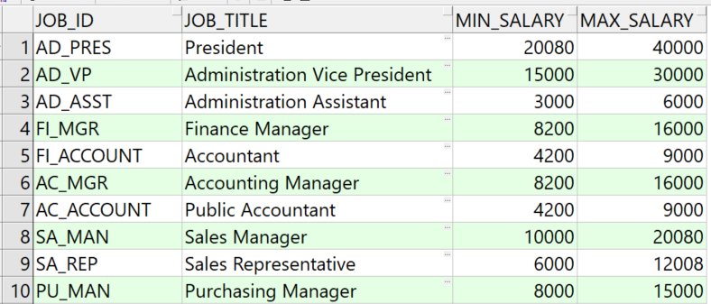
The structure of jobs table and the sample data are as follows:

Processing method:
Retrieve the JOB_ID field values of jobs table and sort them to a job sequence. Add JOB_NUM field to customer wide table to store the sequence number of JOB_ID in job sequence.
3. Date integerization
Most of the time, date data are only used for comparison without the need to calculate the interval, so they can be stored as small integers. It is more common to calculate by year and month in multidimensional analysis, and the small-integerizated date requires the year and month can be easily extracted out.
Processing method:
Instead of saving date data to composite table, we can calculate the number of months between the BEGIN_DATE field value and a beginning date, multiply it by 100 and add the day value of BEGIN_DATE to it, saving that result to the composite table. The beginning date is determined by the distribution characteristics of the date data, and the larger the value, the better.
For example: if we find that all the BEGIN_DATEs are after year 2000, then we can set the beginning date as 2000-01-01.
We can convert the field value of BEGIN_DATE in the customer wide table after the beginning date has been set. For example: when BEGIN_DATE is 2010-11-20, we first calculate that the difference number of months between it and the beginning date 2000-01-01 is 130, multiply it by 100 and add the day value 20 to get the small integer 13020.
With 2000-01-01 as the beginning date, the values after integerization are all less than 65536 when BEGIN_DATE is less than year 2050. As we can see, the beginning date should be as late as the business data allow, so that we can avoid the situations that the date in the wide table are out of the range of small integers to a greater extent.
4. Unintegerization cases
Fields that must be presented as strings such as FIRST_NAME, JOB_TITLE, etc.
Fields that must be presented as floating point numbers such as amounts, discount rates and other fields with decimal parts.
Fields that must be presented as strings concatenated with integers together like international phone numbers.
Processing method:
Keep the original fields unchanged.
Based on the above requirements, modify etl.dfx to retrieve data form the database, and generate a composite table to store the basic wide table after date type conversion. And the code sample is:
A |
B |
|
1 |
=connect@l("oracle") |
=A1.cursor@d("select * from customer") |
2 |
=A1.query@d("select job_id from jobs order by job_id") |
=file("data/job.btx").export@z(A2) |
3 |
=A2.(job_id) |
=date("2000-01-01") |
4 |
=B1.new(int(customer_id):customer_id,first_name,last_name,phone_number,int(interval@m(B3,begin_date)*100+day(begin_date)):begin_date,A3.pos@b(job_id):job_num,job_title,float(balance):balance,int(employee_id):employee_id,int(department_id):department_id,department_name,int(flag1):flag1,int(flag2):flag2,int(flag3):flag3,int(flag4):flag4,int(flag5):flag5,int(flag6):flag6,int(flag7):flag7,int(flag8):flag8) |
|
5 |
=file("data/customer.ctx").create@y(customer_id,first_name,last_name,phone_number,begin_date,job_num,job_title,balance,employee_id,department_id,department_name,flag1,flag2,flag3,flag4,flag5,flag6,flag7,flag8) |
|
6 |
=A5.append(A4) |
>A5.close(),A1.close() |
A1: connect to the pre-configured oracle database, and @l indicates that the retrieved filed names are lowercase. Please note here l is the lowercase L.
B1: create a cursor based on the database, preparing to retrieve the data of customer table. customer is a fact table which is usually big in practice, so it needs to be retrieved with cursor to avoid memory overflowing. The @d option of the cursor is used to convert the “numeric” data type of oracle to “double” data type rather than “decimal” data type. Because “decimal” type of data performs badly in java.
A2: read jobs table from the database, read only the JOB_ID field and sort it. “jobs” is a dimensional table, which is usually small, so it can be loaded in memory directly.
B2: save the data of A2 as a bin file to be used later.
A3: convert A2 to a sequence.
B3: define the date 2000-01-01.
A4: use the “new” function to define three calculations.
1. Convert values like CUSTOMER_ID that are integers for sure from “double” or “string” to “int” with the int function directly converting the type. Please note that “int” should be no greater than 2147483647. For fact tables with more data than this value, the primary key of the sequence number should be of “long” type.
2. Convert JOB_ID from strings to integers to improve the performance. The method is using pos function to get the sequence number of job_id in A3 and define it as JOB_NUM field.
3. Use “interval” to calculate the difference number of months between begin_date and 2000-01-01, multiply it by 100 and add the day value of begin_date. Use “int” to convert the result as integer and save it as new begin_date.
A5: define a composite table file in columnar storage, and the field name is identical to A4.
A6: calculate cursor A4 while exporting to composite table.
B6: close the composite table and the database connection.
When the data volume is ten million, the exported composite table is about 344 MB. The comparison with the file without data type optimization in first issue is as follows:
Number of issue |
Size of file |
Description |
Note |
One |
3.5GB |
Directly exported from database without optimization |
|
Two |
3.0GB |
Data type optimization completed |
We can clearly see from the above table that the file size decreases by 12% (49M) after completing the data type optimization. Smaller files will reduce the amount of reading data from disk, thus effectively improving the performance.
Access wide table
As described previously, many fields of wide table have been optimized, which makes them can not to be queried with the original SQL. We can submit parameters like filtering condition, grouping field, etc. to backend script, and execute the script to convert the parameter value to adapt to optimized data type, then calculate based on the composite table. This method will ensure the parameters passed from the multidimensional analysis front-end remain unchanged. Finally, the calculation results also need to be converted to the corresponding display values.
For example: the given parameter flag1='1' needs to be converted to flag1=1; the jon_num and begin_date in the results also need to be converted from integers to job_id string and date.
Step one: write init.dfx to load the global variable.
To perform this calculation, we need to first write init.dfx file in the main path of node server to pre-load the global variable job for later conversion.
The init.dfx code is as follows:
A |
B |
|
1 |
=file("data/job.btx").import@ib() |
=env(job,A1) |
A1: retrieve the data of bin file, and @i is used to read them as a sequence if there is only one column.
B1: save global variable job.
The written init.dex should be put in the main path of node, and it can be called automatically when the node is started or restarted.
Step two: modify customer.dfx.
The purpose of modification is to add code to convert the parameter value to adapt to optimized data type, and add code for the preparation of converting the result set to strings of display value.
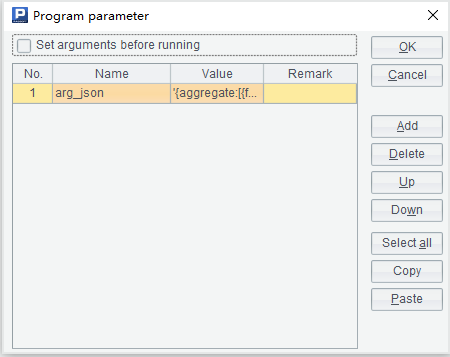
The parameter setup window is exactly the same as the last issue:

The sample of arg_json parameter value remains the same as well:
{
       aggregate:
              [
                     {
                            func:"sum",
                            field:"balance",
                            alias:"sum"
                     },
                     {
                            func:"count",
                            field:"customer_id",
                            alias:"count"
                     }
              ],
       group:
              [
                     "department_id",
                     "job_id",
                     "begin_yearmonth"
              ],
       slice:
              [
                     {
                            dim:"department_id",
                            value:[10,20,50,60,70,80]
                     },
                     {
                            dim:"job_id",
                      value:["AD_VP","FI_MGR","AC_MGR","SA_MAN","SA_REP"]
                     },
                     {
                            dim:"begin_date",
                            interval:[date("2002-01-01"),date("2020-12-31")]
                     },
                     {
                            dim:"flag1",
                            value:"1"
                     },
                     {
                            dim:"flag8",
                            value:"1"
                     }
              ]
}
The customter.dfx will return five strings, respectively the four strings in last issue: “the field names used in the calculation”, aggregate expression, grouping expression and slice (filtering conditions) expression, and a conversion expression of result set display value.
The SPL code is modified as:
A |
B |
C |
|
1 |
func |
||
2 |
if A1.value==null |
return "between("/A1.dim/","/A1.interval(1)/":"/A1.interval(2)/")" |
|
3 |
else if ifa(A1.value) |
return string(A1.value)/".contain("/A1.dim/")" |
|
4 |
else if ifstring(A1.value) |
return A1.dim/"==\""/A1.value/"\"" |
|
5 |
else |
return A1.dim/"=="/A1.value |
|
6 |
=json(arg_json) |
=date("2000-01-01") |
|
7 |
=A6.aggregate.(~.func/"("/~.field/"):"/~.alias).concat@c() |
||
8 |
=A6.group.(if(~=="job_id","job_num",~)) |
||
9 |
=A8.(if(~=="begin_yearmonth","begin_date\\100:begin_yearmonth",~)).concat@c() |
||
10 |
=A6.aggregate.(field) |
=A8.(if(~=="begin_yearmonth","begin_date",~)) |
|
11 |
=(A10|C10).id().concat@c() |
||
12 |
=[] |
||
13 |
for A6.slice |
if A13.dim=="begin_date" && A13.value!=null |
>A13.value=int(interval@m(C6,A13.value)*100+day(A13.value)) |
14 |
else if A13.dim=="begin_date" && A13.value==null |
=A13.interval.(~=int(interval@m(C6,eval(~))*100+day(eval(~)))) |
|
15 |
else if A13.dim=="job_id" |
>A13.dim="job_num" |
|
16 |
>A13.value=A13.value.(job.pos@b(~)) |
||
17 |
else if like(A13.dim, "flag?") |
>A13.value=int(A13.value) |
|
18 |
=[func(A1,A13)] |
>A12|=B18 |
|
19 |
=A6.group|A6.aggregate.(alias) |
=A19(A19.pos("job_id"))="job(job_num):job_id" |
|
20 |
=A19(A19.pos("begin_yearmonth"))="month@y(elapse@m(date(\""/C6/"\"),begin_yearmonth)):begin_yearmonth" |
||
21 |
=A19(A19.pos("begin_date"))="elapse@m(B4,begin_date\\100)+(begin_date%100-1):begin_date" |
||
22 |
return A11,A7,A9,A12.concat("&&"),A19.concat@c() |
||
Area from A1 to C5 is a subprogram which executes only when being called. We will explain them in the order of execution for the sake of better illustration.
A6: parse arg_json to table sequence. The result returned is a nested multi-layer table sequence as follows:

The “aggregate” in it is:

The “group” is:

And the “slice” is:

C6: define the beginning date as 2000-01-01 for the conversion of date values in parameters and results.
A7: first calculate “aggregate” to a string sequence concatenated by colon, and then concatenate the sequence with commas to a string: sum(balance):sum,count(customer_id):count, i.e. the aggregate expression.
A8: replace the job_id in “group” with job_num.
A9: replace the begin_yearmonth in A8 with expression begin_date\100:begin_yearmonth. And concatenate the members of A8 to a string with commas: department_id,job_num,begin_date\100:begin_yearmonth, i.e. the grouping expression.
A10: get the “field” in "aggregate", i.e., all the field names used in aggregate expression.
C10: replace begin_yearmonth in “group” with begin_date and the results are all the field names used in grouping expression.
A11: concatenate A10 and C10 together and continue to concatenate it with commas to a string in order to get all the required field names of the calculation: balance,begin_date,customer_id,department_id,job_num.
A12: define an empty sequence which prepares to store the sequence of slice (filtering conditions) expression.
A13: loop through “slice” and the loop body is the area from B13 to C18 in which B13 to C17 is the optimization conversion to the “value” or “interval” of “slice”.
B13: if the “dim” of A13 (the current slice) is begin_date and the “value” is not null, that is, the begin_date equals to the specified date like begin_date==date("2010-11-01"). In this case, C13 calculates the converted integer value of date("2010-11-01") and assigns it to the “value” of A13.
B14: if the “dim” of A13 is begin_date and the “value” is null, that is, the begin_date is between the two dates such as begin_date is between date("2002-01-01") and date("2020-12-31"). In this case, C14 calculates the converted integer values of these two dates and assigns them to two members of “interval” in A13.
B15: if the “dim” of A13 is job_id, that is, job_id is of enumeration value, for example, ["AD_VP","FI_MGR","AC_MGR","SA_MAN","SA_REP"].contain(job_id). In this case, C15 converts the “dim” of A13 to job_num and C16 converts the enumeration value “value” of A13 to the position in the sequence of global variable “job”, i.e., job_num integer sequence. For example: [5,7,2,15,16].
B17: if the “dim” of A13 is flag1, flag2, ..., flag8, that is, the flag bit equals to “1” or “0”. In this case, C17 converts the “value” of A13 from strings to integers.
B18: take the result of B13 to C17, which convert the “value” or “interval” of “slice” for performance optimization, as parameter to call subprogram A1.
The subprogram A1 (from B2 to B5) is identical to the func code in last issue, which will not be elaborated here.
C18: append the return result of func A1 to A12. Continue the loop in A13 until it is over.
A19: prepare the conversion expression of result set display value from here. Concatenate A6.group with A6.aggregate.alias sequence as follows:

C19: replace the job_id in A19 with conversion statement which is used to convert the job_num in result set to job_id.
A20: replace the begin_yearmonth in A19 with conversion statement which is used to convert the begin_yearmonth integers in grouping fields to yyyymm.
A21: replace the begin_date in A19 with conversion statement which is used to convert the integerized date values to date data. At this point, A19 is the prepared result set display value conversion expression:

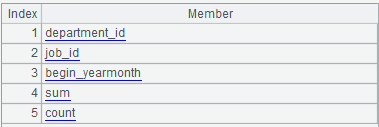
A13: return A10, A7, A8, A11.concat("&&") and A19.concat@c() respectively as:
The field names used in the calculation:
balance,begin_date,customer_id,department_id,job_num
The aggregate expression: sum(balance):sum,count(customer_id):count
Th grouping expression: department_id,job_num,begin_date\100:begin_yearmonth
The slice expression: [10,20,50,60,70,80].contain(department_id)
&& [5,7,2,15,16].contain(job_num) && between(begin_date,2401:25131)
&& flag1==1 && flag8==1
The result set display value conversion expression: department_id,job(job_num):job_id,month@y(elapse@m(date("2000-01-01"),begin_yearmonth)):begin_yearmonth,sum,count
Step three: modify olap.dfx.
We should modify olap.dfx according to the requirements of data type optimization, adding code to convert the calculation result to corresponding display value.
The parameters of olap.dfx are still arg_table and arg_json.
The modified SPL code is as follows:
A |
|
1 |
=call(arg_table/".dfx",arg_json) |
2 |
=file("data/"/arg_table/".ctx").open() |
3 |
=A2.cursor@m(${A1(1)};${A1(4)};2) |
4 |
=A3.groups(${A1(3)};${A1(2)}) |
5 |
=A4.new(${A1(5)}) |
6 |
return A5 |
A5 is added to the code, but all else remains the same.
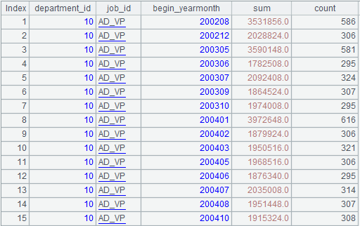
A5: convert the result of A4 to display value and the statement actually executed is :
=A4.new(department_id,job(job_num):job_id,month@y(elapse@m(date("2000-01-01"),begin_yearmonth)):begin_yearmonth,sum,count)。
The execution result is:

A6: return the result set of A5.
After being written, olap-spl.dfx can be called as a stored procedure during multidimensional analysis, and the Java code is the same as that in last issue:
public void testOlapServer(){
       Connection con = null;
       java.sql.PreparedStatement st;
       try{
              // create a connection
              Class.forName("com.esproc.jdbc.InternalDriver");
              // get the connection based on url
              con= DriverManager.getConnection("jdbc:esproc:local://?onlyServer=true&sqlfirst=plus");
              // call the stored procedure, and olap is the file name of dfx
st =con.prepareCall("call olap(?,?)");
st.setObject(1, "customer");
st.setObject(2, "{aggregate: [{func:\"sum\",field:\"balance\",alias:\"sum\"},{func:\"count\",field:\"customer_id\",alias:\"count\"}],group:[\"department_id\",\"job_id\",\"begin_yearmonth\"],slice:[{dim:\"department_id\",value:[10,20,50,60,70,80]},{dim:\"job_id\",value:[\"AD_VP\",\"FI_MGR\",\"AC_MGR\",\"SA_MAN\",\"SA_REP\"]},{dim:\"begin_date\",interval:[date(\"2002-01-01\"),date(\"2020-12-31\")]},{dim:\"flag1\",value:\"1\"},{dim:\"flag8\",value:\"1\"}]}");//arg_json
// execute the stored procedure
st.execute();
// get the result set
ResultSet rs = st.getResultSet();
// continue to process the result set and show it out

       }
       catch(Exception e){
              out.println(e);
       }
       finally{
              // close the connection
              if (con!=null) {
                     try {con.close();}
                     catch(Exception e) {out.println(e);       }
              }
       }
}
Compare the total execution time of Java code plus the backend calculation of return results to that of the first issue as follows:
Number of issue |
Single-thread |
Two-thread |
Note |
One |
84 seconds |
42 seconds |
|
Two |
31 seconds |
14 seconds |
As elaborated in last issue, the execution time in the above table is related to the hardware environments and the absolute values are not important. What matters is that the comparison in the table shows that the data type optimization effectively improves the computational performance.
SPL Official Website 👉 https://www.scudata.com
SPL Feedback and Help 👉 https://www.reddit.com/r/esProcSPL
SPL Learning Material 👉 https://c.scudata.com
SPL Source Code and Package 👉 https://github.com/SPLWare/esProc
Discord 👉 https://discord.gg/cFTcUNs7
Youtube 👉 https://www.youtube.com/@esProc_SPL


Chinese version