Abstract

This series of articles explain how to perform multidimensional analysis (OLAP) in steps with detailed samples. Click to learn more in Multidimensional Analysis Backend Practice 5: small fact table associate with small dimension table. Multidimensional Analysis Backend Practice 5: small fact table associate with small dimension table

Aim of practice

This issue aims to associate the new customer data of the latest day in the customer wide table with multiple dimension tables such as the branch department table, and perform slice and grouping calculation with dimension table fields on the basis of previous calculations.

 

The steps of practice are:

1. Prepare dimension tables such as branch department table: retrieve the data of branch department table and so on from the database and save as a bin file.

2. Associate the new customer data in wide table with the dimension tables, and perform slice and grouping calculations: implemented by calling SPL with Java code.

 

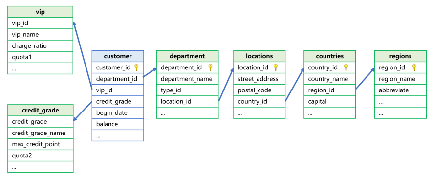
The associations between the customer table and each dimension table are shown in the picture:

 

The dimension tables include:

1. The branch department table “department”

The SQL statement for retrieving dimension table data form Oracle database is select * from department. And its execution result is:

 

 The fields include:

       DEPARTMENT_ID NUMBER(4,0) id number of branch department
       DEPARTMENT_NAME VARCHAR2(32) name of branch department
       MANAGER_ID NUMBER(6,0) id number of manager
       LOCATION_ID NUMBER(4,0) id number of location
       TYPE_ID NUMBER(6,0) id number of type
       APPLAUSE_RATE NUMBER(3,0) applause rate
       OPENING_DATE DATE opening date
       STAR NUMBER(1,0) star classification
       ENTERPRISE_TYPE_ID NUMBER(6,0) enterprise type
       MAIN_BUSINESS NUMBER(6,0) main business

2. The location table “location”

The fields include:

LOCATION_ID NUMBER(4,0) id number of location
STREET_ADDRESS VARCHAR2(40) street address
POSTAL_CODE VARCHAR2(12) postal code
CITY VARCHAR2(30) city
STATE_PROVINCE VARCHAR2(25) state or province
COUNTRY_ID CHAR(2) id number of country

3. The country table “countries”

COUNTRY_ID CHAR(2) id number of country
COUNTRY_NAME VARCHAR2(40) name of country
REGION_ID NUMBER id number of region
CAPITAL VARCHAR2(40) capital

4. The region table “regions”

REGION_ID NUMBER id number of region
REGION_ID_NAME VARCHAR2(40) name of region
abbreviate VARCHAR2(10) abbreviation of name

5. The VIP table “vip”

VIP_ID NUMBER(4,0)VIP id number of VIP 
VIP_NAME VARCHAR2(30) name of VIP
MAX_POINT NUMBER(6,0) maximum point
MIN_POINT NUMBER(6,0) minimum point
CHARGE_RATIO NUMBER(4,0) ratio of charge (3-10)
INTEREST_RATE1 NUMBER(4,0) interest rate of cash withdrawal (8-15)
QUOTA1 NUMBER(8,0) quota of quick cash withdrawal (1000-8000)
QUOTA2 NUMBER(8,0) quota of free repayment (10000-160000)
NUMBER1 NUMBER(2,0) number of quick boarding per month(0-3)
NUMBER2 NUMBER(2,0) number of high-speed rail VIP room per month(0-3)

6. The credit grading table “credit_grade”

CREDIT_GRADE NUMBER(4,0) credit grade
CREDIT_GRADE_NAME VARCHAR2(30) name of credit grade
MAX_CREDIT_POINT NUMBER(6,0) maximum of credit point
MIN_CREDIT_POINT NUMBER(6,0) minimum of credit point
QUOTA1 NUMBER(8,0) quota of payment(10000-90000)
QUOTA2 NUMBER(8,0) quota of cash withdrawal(10000-90000)
QUOTA3 NUMBER(8,0) quota of password-free payment(1000-9000)

The purpose of multidimensional analysis calculation can be described in the following SQL statement of Oracle:

select v.interest_rate1,ct.country_id,c.job_id,sum(c.balance) sum,count(c.customer_id) count
from customer c
 left join department d on c.department_id=d.department_id
 left join locations l on d.location_id=l.location_id
 left join countries ct on l.country_id=ct.country_id
 left join regions r on r.region_id=ct.region_id
 left join vip v on c.vip_id=v.vip_id
 left join credit_grade cg on c.credit_grade=cg.credit_grade
where d.applause_rate between 5 and 95
and r.region_name in ('Asia','Europe','Americas')
and v.charge_ratio between 9 and 11
and cg.quota2 between 50000 and 80000
and c.job_id in ('AD_VP','FI_MGR','AC_MGR','SA_MAN','SA_REP')
and c.flag1='1' and c.flag8='1'
group by v.interest_rate1,ct.country_id,c.job_id

Prepare wide table

Continue to write etl.dfx, retrieving dimension tables such as branch department table from the database to generate a bin file. The code sample is:

	A	B	C
1	=connect@l("oracle")
2	=A1.query@d("select   * from department order by department_id")	=A2.new(int(department_id):department_id,department_name,int(manager_id):manager_id,int(location_id):location_id,int(type_id):type_id,int(applause_rate):applause_rate,opening_date,int(star):star,int(enterprise_type_id):enterprise_type_id,int(main_business):main_business)	=file("data/department.btx").export@z(B2)
3	=A1.query@d("select   * from vip order by vip_id")	=A3.new(int(vip_id):vip_id,vip_name,int(max_point):max_point,int(min_point):min_point,int(charge_ratio):charge_ratio,int(interest_rate1):interest_rate1,int(quota1):quota1,int(quota2):quota2,int(number1):number1,int(number2):number2)	=file("data/vip.btx").export@z(B3)
4	=A1.query@d("select   * from credit_grade order by credit_grade")	=A4.new(int(credit_grade):credit_grade,credit_grade_name,int(max_credit_point):max_credit_point,int(min_credit_point):min_credit_point,int(quota1):quota1,int(quota2):quota2,int(quota3):quota3)	=file("data/credit_grade.btx").export@z(B4)
5	=A1.query@d("select   * from locations")	=A5.new(int(location_id):location_id,street_address,postal_code,city,state_province,country_id)	=file("data/locations.btx").export@z(B5)
6	=A1.query@d("select   * from countries")	=A6.new(country_id,country_name,int(region_id):region_id)	=file("data/countries.btx").export@z(B6)
7	=A1.query@d("select   * from regions")	=A7.new(int(region_id):region_id,region_name)	=file("data/regions.btx").export@z(B7)

A1: connect to the pre-configured oracle database. @l option is used to process the file name to lowercase and l is the lowercase L rather than number 1.

A2: retrieve the data in the “department” table which is a dimension table with small size in practice and can be fully loaded in memory.

B2: small integerize the fields as much as possible to decrease the memory occupation.

C2: store the converted data in the bin file.

A3-C3: read, process and store the data in “vip” table.

A4-C3: read, process and store the data in “credit_grade” table.

A5-C5: read, process and store the data in “locations” table.

A6-C6: read, process and store the data in “countries” table.

A7-C7: read, process and store the data in “regions” table.

 

Pre-process data

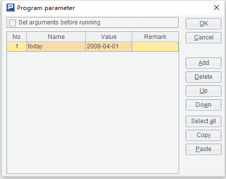
The new customer data of one day is not too many, which can be loaded in memory completely. So we can continue to write init.dfx, loading new customers and each dimension table in memory, and the cellset parameter is “today” (the current date).

 

The code is as follows:

	A	B
1	=file("data/job.btx").import@ib()	>env(job,A1)
2	=file("data/department.btx").import@b().keys(department_id)	=file("data/vip.btx").import@b().keys(vip_id)
3	=file("data/credit_grade.btx").import@b().keys(credit_grade)	=file("data/locations.btx").import@b().keys(location_id)
4	=file("data/countries.btx").import@b().keys(country_id)	=file("data/regions.btx").import@b().keys(region_id)
5	=A2.switch(location_id,B3.switch(country_id,A4.switch(region_id,B4)))
6	=file("data/customer_begin_date.ctx").open().cursor(department_id,job_num,employee_id,customer_id,first_name,last_name,phone_number,job_title,balance,department_name,flag1,flag2,flag3,flag4,flag5,flag6,flag7,flag8,vip_id,credit_grade;begin_date==if(ifdate(today),today,now())).fetch()
7	=A6.join(department_id,A2,~:department_detail;vip_id,B2,~:vip_detail;credit_grade,A3,~:credit_grade_detail)
8	>env(newCustomer,A7)

A1: retrieve the data of job in the bin file, @i is used to read them as a sequence if there is only one column.

B1: save as global variable “job”.

A2-B4: retrieve the data of branch department, vip, credit grading, location, country, and region in the bin file respectively, and create primary keys.

A5: associate the “department”, “locations”, “countries” and “regions” tables according to their layers.

A6: retrieve today’s new customer data from the composite table customer_begin_date.ctx without the begin_date field. If “today” is not a date parameter (or is null), then the current date is used instead.

A7: copy the new customer data department_id field to department_detail and associate it with the global variable “department”. Process “vip” and “credit_grade” in the same way.

A8: save the associated new customer data as global variable “newCustomer”.

 

The written init.dfx should be put in the main path of node, and it can be called automatically when the node is started or restarted.

 

init.dfx should also be executed when adding new customer data every day in order to update newCustomer. We should continue to write etlAppend.dfx, and use ETL tools or OS timed tasks to invoke etlAppend.dfx script from the command line.

 

For example:

C:\Program Files\raqsoft\esProc\bin>esprocx etlAppend.dfx.dfx

 

The cellset and code in etlAppend.dfx are as follows:

 

	A
1	=connect@l("oracle")
2	=A1.cursor("select * from customer where begin_date=?",today)
3	=file("data/customer_begin_date.ctx").open().append(A2)
4	>A3.close(),A1.close()
5	>callx("init.dfx",today;["localhost:8281"])

Area from A1 to A4 keeps unchanged.

A5: call the init.dfx in the node, and the cellset is “today”.

 

Associate calculation

The olap.dfx in previous issues can not be directly used here because of the different syntax of in-memory and external storage calculations. Instead, we need to write another olapMem.dfx.

 

There are still two given parameters: the value of table name arg_table is newCustomer, and other parameters are in json format. The arg_json smaple is as follows:

{
       aggregate:
              [
                     {
                            func:"sum",
                            field:"balance",
                            alias:"sum"
                     },
                     {
                            func:"count",
                            field:"customer_id",
                            alias:"count"
                     }
              ],
       group:
              [
                    "vip_detail.interest_rate1:vip_detail_interest_rate1",
               "department_detail.location_id.country_id.country_id:department_detail_location_id_country_id",
                     "job_id"
              ],
       slice:
              [
                     {
                            dim:"department_detail.applause_rate",
                            interval:[10,95]
                     },
                     {
                      dim:"department_detail.location_id.country_id.region_id.region_name",
                            value:["Asia","Europe","Americas"]
                     },
                     {
                            dim:"vip_detail.charge_ratio",
                            interval:[9,11]
                     },
                     {
                            dim:"credit_grade_detail.quota2",
                            interval:[50000,80000]
                     },
                     {
                            dim:"job_id",
                      value:["AD_VP","FI_MGR","AC_MGR","SA_MAN","SA_REP"]
                     },
                     {
                            dim:"flag1",
                            value:"1"
                     },
                     {
                            dim:"flag8",
                            value:"1"
                     }
              ]
}

The reason why there are department_detail.location_id, department_detail.applause_rate, etc. in “group” and “slice” is that data pre-processing adopts to the foreign key attribute in advance. Therefore, we can directly use department_detail to retrieve the different attributions of each branch department.

 

The colon in department_detail.location_id.country_id.country_id:department_detail_location_id_country_id is used to give an alias for the foreign key attribute field, which is used as the field name of the final result. The reason why there is country_id.country_id in the field is that the first country_id has already been attributed as foreign key, that is, has become a reference that can not be returned to front-end directly. While the second one is a single value which can be returned directly to front-end.

 

Step one: write newCustomer.dfx.

 

Before writing olapMem.dfx, we should first rewrite customer.dfx to newCustomer.dfx in order to process the parameter arg_json, and the SPL code is as follows:

	A	B	C
1	func
2		if A1.value==null	return "between("/A1.dim/","/A1.interval(1)/":"/A1.interval(2)/")"
3		else if ifa(A1.value)	return   string(A1.value)/".contain("/A1.dim/")"
4		else if   ifstring(A1.value)	return   A1.dim/"==\""/A1.value/"\""
5		else	return   A1.dim/"=="/A1.value
6	=json(arg_json)
7	=A6.aggregate.(~.func/"("/~.field/"):"/~.alias).concat@c()
8	=A6.group.(if(~=="job_id","job_num",~)).concat@c()
9	=[]
10	for A6.slice	if   A10.dim=="job_id"	>A10.dim="job_num"
11			>A10.value=A10.value.(job.pos@b(~))
12		else if like(A10.dim,   "flag?")	>A10.value=int(A10.value)
13		=[func(A1,A10)]	>A9|=B13
14	=A6.group.(~.split(":")).(~=~.m(-1))|A6.aggregate.(alias)		=A14(A14.pos("job_id"))="job(job_num):job_id"
15	return   A7,A8,A9.concat("&&"),A14.concat@c()

Area from A1 to C5 is subprogram which only executes when being called. The code is exactly the same as customer.dfx.

 

A6: parse arg_json to a table sequence and the return result is a nested multi-layer table sequence as follows:

 

The “aggregate” in it is:

 

The “group” is:

 

The “slice” is:

 

A7: first calculate “aggregate” to colon-concatenated string sequences and then concatenate the sequences to a string with comma: sum(balance):sum,count(customer_id):count, i.e., the aggregate expression.

 

A8: replace the job_id in “group” with job_num.

 

A9: define an empty sequence which prepares to store the slice (filtering conditions) expressions.

 

A10: loop through “slice” and the loop body is the area from B10 to C13 in which from B10 to C12 is the optimization conversion to the “value” or “interval” of “slice”.

 

B10: if the “dim” of A10 is job_id, that is, job_id is of enumeration value, for example, ["AD_VP","FI_MGR","AC_MGR","SA_MAN","SA_REP"].contain(job_id). In this case, C10 converts the “dim” of A10 to job_num and C11 converts the enumeration value “value” of A10 to the position in the sequence of global variable “job”, i.e., job_num integer sequence. For example: [5,7,2,15,16].

 

B12: if the “dim” of A10 is flag1, flag2, ..., flag8, that is, the flag bit equals to “1” or “0”. In this case, C12 converts the “value” of A10 from strings to integers.

 

B13: take the result of B10 to C13, which converts the “value” or “interval” of “slice” for performance optimization, as parameter to call subprogram A1.

 

The subprogram A1 (from B2 to B5) is identical to the func code in the first issue, which will not be elaborated here.

 

C13: append the return result of func A1 to A9. Continue the loop in A10 until it is over. And the sequence of slice expressions is well prepared.

 

A14: prepare the conversion expression of result set display value. Concatenate A6.group.(~.split(":")).(~=~.m(-1)) with A6.aggregate.alias sequence as follows:

 

A6.group.(~.split(":")).(~=~.m(-1)) is used to take the alias after the colon if there is one in the “group”, otherwise the value of “group” is directly taken.

 

C14: replace the job_id in A19 with conversion statement which is used to convert the job_num in result set to job_id.

 

A15: return A7, A8, A9.concat("&&") and A14.concat@c() respectively as:

The aggregate expression:

vip_detail.interest_rate1:vip_detail_interest_rate1,

department_detail.location_id.country_id:department_detail_location_id_ country_id,

job_num

The slice expression:

between(department_detail.applause_rate ,10:95)

&&["Asia","Europe","Americas"].contain(department_detail.location_id.country_id.region_id.region_name)

&& between(vip_detail.charge_ratio,9:11)

&& between(credit_grade_detail.quota2,50000:80000)

&& [5,7,2,15,16].contain(job_num)

&& flag1==1 && flag8==1

The result set display value conversion expression:

vip_detail_interest_rate1,department_detail_location_id_country_id,job(job_num):job_id,sum,count

 

Step two: write olapMem.dfx.

 

The cellset parameters are arg_table (whose value is newCustomer) and arg_json. The SPL code is as follows:

	A
1	=call(arg_table/".dfx",arg_json)
2	=${arg_table}.select(${A1(3)})
3	=A2.groups(${A1(2)};${A1(1)}).new(${A1(4)})
4	return A3

 

A1: call newCustomer.dfx based on the value of parameter arg_table, the calling parameter is arg_json, and the return value is the four expression strings returned by newCustomer.

 

A2: calculate the slice expression on global variable “newCustomer” table sequence to achieve data filtering based on the parameter arg_table. The SPL statement actually executed is:

newCustomer.select(between(department_detail.applause_rate ,10:95) && ["Asia","Europe","Americas"].contain(department_detail.location_id.country_id.region_id.region_name) && between(vip_detail.charge_ratio,9:11) && between(credit_grade_detail.quota2,50000:80000) && [5,7,2,15,16].contain(job_num) && flag1==1 && flag8==1)

 

A3: perform grouping and aggregation on A2 and rename the result according to alias. And the statement actually executed is:

=A2.groups(vip_detail.interest_rate1:vip_detail_interest_rate1,department_detail.location_id.country_id.country_id:department_detail_location_id_country_id,job_num; sum(balance):sum,count(customer_id):count).new(vip_detail_interest_rate1,department_detail_location_id_country_id,job(job_num):job_id,sum,count)

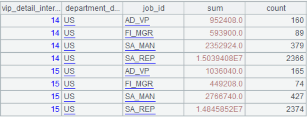
The execution result is:

 

 

Step three: call with Java code

 

After being written, olapMem.dfx can be called as a stored procedure during multidimensional analysis, and most of the Java code is the same as those in previous issues with differences in the name of dfx file, and the values of arg_table and arg_json. The Java code is:

public void testOlapServer(){
       Connection con = null;
       java.sql.PreparedStatement st;
       try{
              // create a connection
              Class.forName("com.esproc.jdbc.InternalDriver");
              // get the connection based on url
              con= DriverManager.getConnection("jdbc:esproc:local://?onlyServer=true&sqlfirst=plus");
              // call the stored procedure, and olap is the file name of dfx
st =con.prepareCall("call olapMem(?,?)");
st.setObject(1, "newCustomer");
st.setObject(2, "{aggregate:[{func:\"sum\",field:\"balance\",alias:\"sum\"},{func:\"count\",field:\"customer_id\",alias:\"count\"}],group:[\"vip_detail.interest_rate1:vip_detail_interest_rate1\",\"department_detail.location_id.country_id:department_detail_location_id_country_id\",\"job_id\"],slice:[{dim:\"department_detail.applause_rate\",interval:[10,95]},{dim:\"department_detail.location_id.country_id.region_id.region_name\",value:[\"Asia\",\"Europe\",\"Americas\"]},{dim:\"vip_detail.charge_ratio\",interval:[9,11]},{dim:\"credit_grade_detail.quota2\",interval:[50000,80000]},{dim:\"job_id\",value:[\"AD_VP\",\"FI_MGR\",\"AC_MGR\",\"SA_MAN\",\"SA_REP\"]},{dim:\"flag1\",value:\"1\"},{dim:\"flag8\",value:\"1\"}]}");//arg_json
// execute the stored procedure
st.execute();
// get the result set
ResultSet rs = st.getResultSet();
// continue to process the result set and show it out
             
       }
       catch(Exception e){
              out.println(e);
       }
       finally{
              // close the connection
              if (con!=null) {
                     try {con.close();}
                     catch(Exception e) {out.println(e);       }
              }
       }
}

The total execution time of Java code plus SPL is 0.3 seconds.